As more and more enterprise data is stored, the contradiction between storage capacity, query performance, and storage cost is a common problem for technical teams. This problem is particularly prominent in the two scenarios of Elasticsearch and ClickHouse. In order to meet the query performance requirements of different hot data, these two components have some strategies for layering data in the architecture design.
At the same time, in terms of storage media, with the development of cloud computing, object storage has won the favor of enterprises due to its low price and elastic expansion space. More and more enterprises migrate warm and cold data to object storage. However, if the index and analysis components are directly connected to the object storage, problems such as query performance and compatibility will occur.
This article will introduce the basic principles of hot and cold data tiering in these two scenarios, and how to use JuiceFS to deal with the problems existing in object storage.
01- Detailed Explanation of Elasticsearch Data Hierarchy
Before introducing how ES implements the hot and cold data layering strategy, let's understand three related concepts: Data Stream, Index Lifecycle Management and Node Role.
Data Stream
Data Stream (data stream) is an important concept in ES, which has the following characteristics:
- Streaming write: it is a stream-written data set, rather than a fixed-size collection;
- Append-only write: it updates the data in the way of append-write, and does not need to modify the historical data;
- Timestamp: Each new piece of data will have a timestamp record when it was generated;
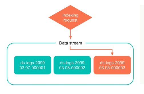
- Multiple indexes: There is an index concept in ES, and each piece of data will eventually fall into its corresponding index, but data flow is a higher-level and larger concept, and there may be many indexes behind a data flow. These indexes are generated according to different rules. Although a data stream is composed of many indexes, only the latest index is writable, and the historical index is read-only, and once solidified, it cannot be modified.
Log data is a type of data that conforms to the characteristics of data streams. It is only appended and written, and it must also have a timestamp. Users will generate new indexes based on different dimensions, such as by day or by other dimensions.
The figure below is a simple example of data flow indexing. During the process of using data flow, ES will directly write to the latest index instead of the historical index, and the historical index will not be modified. As more new data is generated in the future, this index will also precipitate into an old index.
As shown in the figure below, when the user writes data into ES, it is roughly divided into two stages:
- Phase 1: The data will be written to the In-memory buffer buffer of the memory first;
- Phase 2: The buffer falls to the local disk according to certain rules and time, which is the green persistent data in the figure below, which is called Segment in ES.
There may be some time difference during this process. During the persistence process, if you trigger a query, the newly created Segment cannot be searched. Once the Segment is persisted, it can be searched by the upper query engine immediately.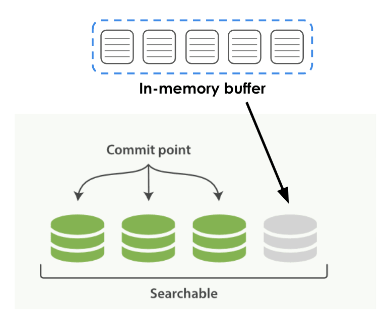
Index Lifecycle Management
Index Lifecycle Management, referred to as ILM, is the index lifecycle management. ILM defines the lifecycle of an index as 5 phases:
- Hot data (Hot): data that needs to be updated or queried frequently;
- Warm data (Warm): data that is no longer updated but still frequently queried;
- Cold data (Cold): data that is no longer updated and has low query frequency;
- Frozen data: Data that is no longer updated and hardly queried. You can safely put this kind of data in a relatively slowest and cheapest storage medium;
- Delete data (Delete): Data that is no longer needed and can be deleted with confidence.
The data in an index, whether it is an index or a segment, will go through these stages. The rules of this classification help users manage the data in ES very well. Users can define rules for different stages by themselves.
Node Role
In ES, each deployment node will have a Node Role, which is the node role. Each ES node will be assigned different roles, such as master, data, ingest, etc. Users can combine node roles and the stages of the different life cycles mentioned above for data management.
Data nodes will have different stages, which may be a node that stores hot data, or a node that stores warm data, cold data, or even extremely cold data. It is necessary to assign different roles to nodes according to their functions, and configure different hardware for nodes with different roles.
For example, for hot data nodes, high-performance CPUs or disks need to be configured. For warm and cold data nodes, it is basically considered that the data is queried less frequently. At this time, the hardware requirements for certain computing resources are actually not so high. .
Node roles are defined according to different stages of the life cycle. It should be noted that each ES node can have multiple roles, and these roles are not in one-to-one correspondence. Here is an example. When configuring in the YAML file of ES, node.roles is the configuration of node roles. You can configure multiple roles for this node according to the roles it should have.
node.roles: ["data_hot", "data_content"]
life cycle policy
After understanding the concepts of Data Stream, Index Lifecycle Management, and Node Role, you can create some different lifecycle policies for data.
According to the index characteristics of different dimensions defined in the life cycle policy, such as the size of the index, the number of documents in the index, and the time when the index was created, ES can automatically help users roll the data of a certain life cycle stage to another stage, The term in ES is rollover.
For example, users can specify features based on the index size dimension, roll hot data to warm data, or roll warm data to cold data according to some other rules. In this way, when the index is rolled between different stages of the life cycle, the corresponding indexed data will also be migrated and rolled. ES can automatically complete these tasks, but the lifecycle policy needs to be defined by the user.
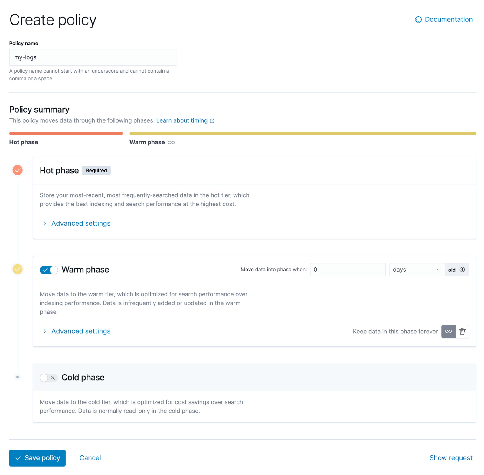
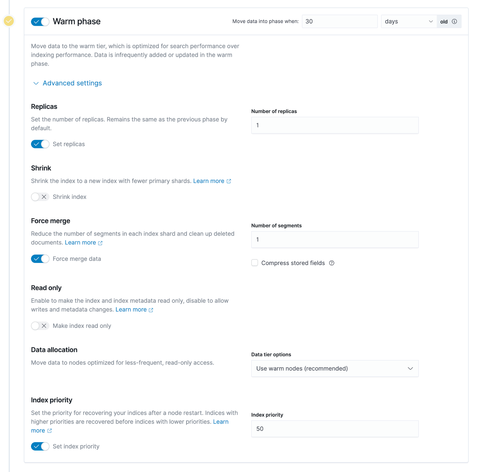
The screenshot below is Kibana's management interface, where users can configure lifecycle policies graphically. It can be seen that there are three stages, from top to bottom are hot data, warm data and cold data.
Expand the advanced settings of the hot data stage, and you can see more details, the above-mentioned policy configuration based on different dimensional characteristics, such as the three options seen on the right side of the figure below.
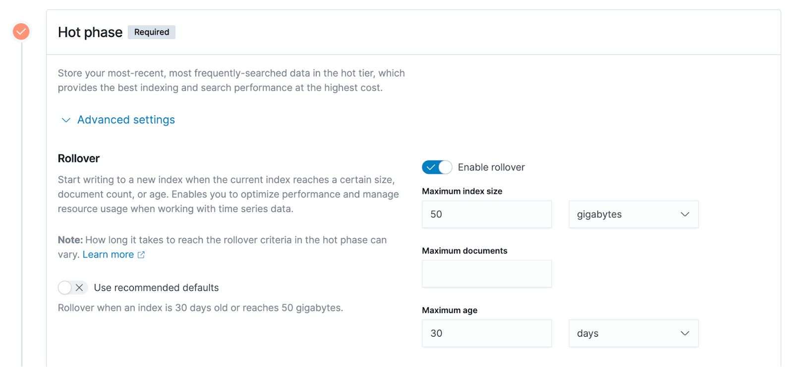
- The size of the index, the example in the diagram is 50GB, when the size of the index exceeds 50GB, it will be rolled from the hot data stage to the warm data stage.
- The maximum number of documents, the index unit in ES is document, and user data is written into ES in the form of document, so the number of documents is also a measurable indicator.
- The maximum index creation time. The example here is 30 days. Suppose an index has been created for 30 days. At this time, the rollover from hot data stage to warm data just mentioned will be triggered.
02- Detailed explanation of ClickHouse data layered architecture
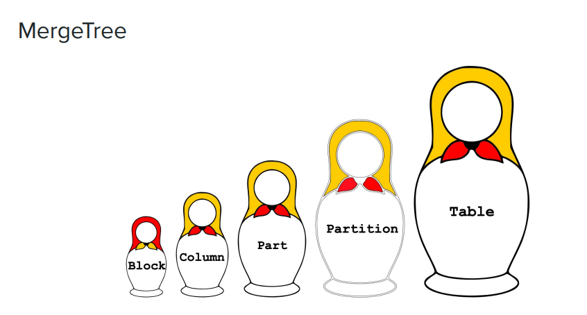
The picture below is a set of Russian nesting dolls from big to small, which vividly shows the data management mode of ClickHouse, the MergeTree engine.
- Table: On the far right of the picture is the largest concept, the first thing users want to create or have direct access to is Table;
- Partition: It is a smaller dimension or smaller granularity. In ClickHouse, data is divided into Partitions for storage, and each Partition will have an identifier;
- Part: In each Partition, it will be further subdivided into multiple Parts. If you look at the data format stored on the ClickHouse disk, you can think that each subdirectory is a Part;
- Column: In the Part, you will see some smaller-grained data, namely Column. ClickHouse's engine uses columnar storage, and all data is organized in columnar storage. You will see many columns in the Part directory. For example, if there are 100 columns in Table, there will be 100 Column files;
- Block: Each Column file is organized according to the granularity of Block.
In the following example, there are 4 subdirectories under the table directory, and each subdirectory is the Part mentioned above.
$ ls -l /var/lib/clickhouse/data/<database>/<table>
drwxr-xr-x  2 test  test 64B Aug  8 13:46 202208_1_3_0
drwxr-xr-x  2 test  test 64B Aug  8 13:46 202208_4_6_1
drwxr-xr-x  2 test  test 64B Sep  8 13:46 202209_1_1_0
drwxr-xr-x  2 test  test 64B Sep  8 13:46 202209_4_4_
In the rightmost column of the diagram, the name of each subdirectory may be preceded by a time, such as 202208, which is a prefix like this, and 202208 is actually the name of the Partition. Partition names are defined by users themselves, but according to conventions or some practices, time is usually used for naming.
For example, the Partition 202208 has two subdirectories, and the subdirectories are Parts. A Partition usually consists of multiple Parts. When the user writes data to ClickHoue, it will be written into the memory first, and then persisted to the disk according to the data structure in the memory. If the data in the same Partition is relatively large, it will become many parts on the disk. ClickHouse officially recommends not to create too many Parts under a Table. It will merge Parts regularly or irregularly to reduce the total number of Parts. The concept of Merge is to merge Part, which is one of the origins of the name of the MergeTree engine.
Let's understand Part through an example. There will be many small files in Part, some of which are meta information, such as index information, to help users find data quickly.
$ ls -l /var/lib/clickhouse/data/<database>/<table>/202208_1_3_0
-rw-r--r--  1 test  test  ?? Aug  8 14:06 ColumnA.bin
-rw-r--r--  1 test  test  ?? Aug  8 14:06 ColumnA.mrk
-rw-r--r--  1 test  test  ?? Aug  8 14:06 ColumnB.bin
-rw-r--r--  1 test  test  ?? Aug  8 14:06 ColumnB.mrk
-rw-r--r--  1 test  test  ?? Aug  8 14:06 checksums.txt
-rw-r--r--  1 test  test  ?? Aug  8 14:06 columns.txt
-rw-r--r--  1 test  test  ?? Aug  8 14:06 count.txt
-rw-r--r--  1 test  test  ?? Aug  8 14:06 minmax_ColumnC.idx
-rw-r--r--  1 test  test  ?? Aug  8 14:06 partition.dat
-rw-r--r--  1 test  test  ?? Aug  8 14:06 primary.id
On the right side of the example, the files prefixed with Column are the actual data files, which are usually larger compared to the meta information. In this example, there are only two columns, A and B, but there may be many columns in the actual table. All these files, including meta information and index information, will work together to help users quickly jump or search between different files.
ClickHouse storage strategy
If you want to stratify hot and cold data in ClickHouse, you will use a lifecycle policy similar to that mentioned in ES, which is called Storage Policy in ClickHouse.
Slightly different from ES, ClickHouse officially does not divide data into different stages, such as hot data, warm data, and cold data. ClickHouse provides some rules and configuration methods, and users need to formulate stratification strategies by themselves.
Each ClickHouse node supports the configuration of multiple disks at the same time, and the storage media can be various. For example, general users will configure SSD disks for ClickHouse nodes for performance; for some warm and cold data, users can store data in lower-cost media, such as mechanical disks. ClickHouse users are unaware of the underlying storage medium.
Similar to ES, ClickHouse users need to formulate storage strategies based on different dimensional characteristics of the data, such as the size of each part subdirectory, the proportion of remaining space on the entire disk, etc. When the conditions set by a certain dimensional characteristic are met, storage will be triggered Execution of the strategy. This strategy will migrate a part from one disk to another. In ClickHouse, multiple disks configured by a node have priority. By default, data will fall on the disk with the highest priority. This enables Part to be transferred from one storage medium to another.
Some SQL commands of ClickHouse, such as MOVE PARTITION/PART commands, can manually trigger data migration, and users can also do some functional verification through these commands. Secondly, in some cases, it may also be desirable to explicitly transfer the part from the current storage medium to another storage medium through manual rather than automatic transfer.
ClickHouse also supports time-based migration policies, a concept independent of storage policies. After the data is written, ClickHouse will trigger the data migration on the disk according to the time set by the TTL attribute of each table. For example, if the TTL is set to 7 days, ClickHouse will write the data in the table more than 7 days from the current disk (such as the default SSD) to another disk with lower priority (such as JuiceFS).
03- Warm and cold data storage: why use object storage + JuiceFS?
After enterprises store warm and cold data on the cloud, the storage cost is greatly reduced compared with the traditional SSD architecture. Enterprises also enjoy the elastic scaling space on the cloud; they do not need to do any operation and maintenance operations for data storage, such as expansion and contraction, or some data cleaning work . The storage capacity required for warm and cold data is much larger than that of hot data, especially as time goes by, a large amount of data that needs to be stored for a long time will be generated. If these data are stored locally, the corresponding operation and maintenance work will be overwhelmed.
However, if data application components such as Elasticsearch and ClickHouse are used on object storage, there will be problems such as poor write performance and compatibility. Enterprises that want to take into account query performance began to look for solutions on the cloud. In this context, JuiceFS is increasingly used in data layered architectures .
Through the following ClickHouse write performance test, you can intuitively understand the performance difference of writing to SSD, JuiceFS and object storage.
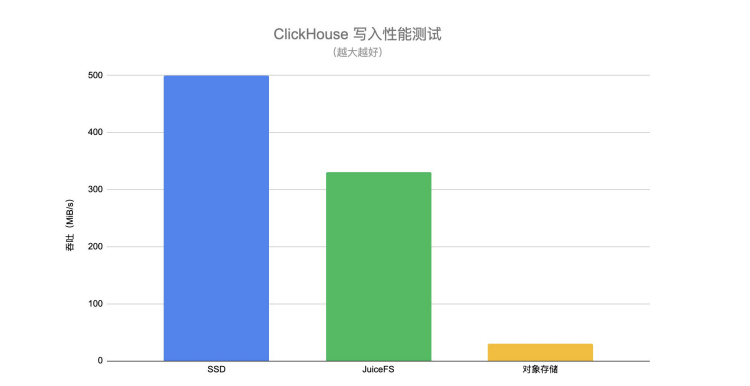
The write throughput of JuiceFS is much higher than that of directly connected object storage and close to that of SSD . When users transfer hot data to the warm data layer, they also have certain requirements for writing performance. During the migration process, if the writing performance of the underlying storage medium is poor, the entire migration process will be dragged on for a long time, which will also bring some challenges to the entire pipeline or data management.
The ClickHouse query performance test in the figure below uses real business data and selects several typical query scenarios for testing. Among them, q1-q4 are queries that scan the entire table, and q5-q7 are queries that hit the primary key index. The test results are as follows:
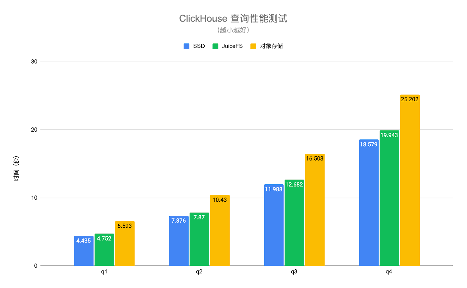
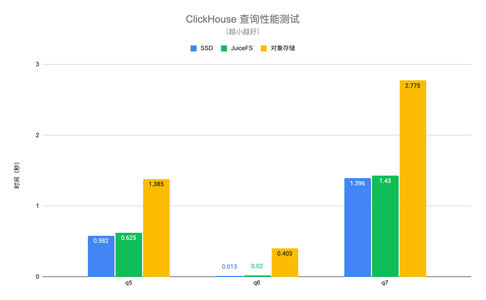
The query performance of JuiceFS and SSD disks is basically the same, with an average difference of about 6%, but the performance of object storage is 1.4 to 30 times lower than that of SSD disks . Thanks to the high-performance metadata operation and local caching features of JuiceFS, the hot data required by the query request can be automatically cached locally on the ClickHouse node, which greatly improves the query performance of ClickHouse. It should be noted that the object storage in the above test is accessed through the S3 disk type of ClickHouse. In this way, only the data is stored on the object storage, and the metadata is still on the local disk. If the object storage is mounted locally in a way similar to S3FS, the performance will be further degraded.
It is also worth mentioning that JuiceFS is a fully POSIX-compatible file system, which is well compatible with upper-layer applications (such as Elasticsearch, ClickHouse). Users are not aware of whether the underlying storage is a distributed file system or a local disk. If object storage is used directly, compatibility with upper-layer applications cannot be achieved well.
04- Practical operation: ES + JuiceFS
Step 1: Prepare multiple types of nodes and assign different roles . Each ES node can be assigned different roles, such as storing hot data, warm data, cold data, etc. Users need to prepare nodes of different models to match the needs of different roles.
Step 2: Mount the JuiceFS file system . Generally, users use JuiceFS for warm and cold data storage. Users need to mount the JuiceFS file system locally on ES warm data nodes or cold data nodes. Users can configure the mount point to ES through symbolic links or other methods, making ES think that its data is stored in a local directory, but behind this directory is actually a JuiceFS file system.
Step 3: Create a lifecycle policy . This needs to be customized by each user. Users can create either through ES API or through Kibana. Kibana provides some relatively convenient ways to create and manage lifecycle policies.
Step 4: Set a lifecycle policy for the index . After creating the lifecycle policy, the user needs to apply this policy to the index, that is, to set the newly created policy for the index. Users can create index templates in Kibana through index templates, or configure them explicitly through API through index.lifycycle.name.
Here are a few tips:
Tip 1: The number of copies (replica) of Warm or Cold nodes can be set to 1 . All data is essentially placed on JuiceFS, and its bottom layer is object storage, so the reliability of the data is already high enough, so the number of copies can be appropriately reduced on the ES side to save storage space.
Tip 2: Turning on Force merge may cause the node CPU to be continuously occupied, so turn it off as appropriate . When transferring from hot data to warm data, ES will merge the underlying segments corresponding to all hot data indexes. If the Force merge function is enabled, ES will first merge these segments, and then store them in the underlying system of warm data. However, merging segments is a very CPU-intensive process. If the data nodes of warm data also need to carry some query requests, you can turn off this function as appropriate, that is, keep the data intact and write it directly to the underlying storage.
Tip 3: Indexes in the Warm or Cold phase can be set to read-only . When indexing warm data and cold data stages, we can basically consider these data to be read-only, and the indexes of these stages will not be modified. Setting it to read-only can properly reduce resources on warm and cold data nodes, such as releasing some memory, thereby saving some hardware resources on warm or cold nodes.
05- Practical operation: ClickHouse + JuiceFS
**Step 1: Mount the JuiceFS file system on all ClickHouse nodes. **This path can be any path, because ClickHouse will have a configuration file to point to the mount point.
**Step 2: Modify the ClickHouse configuration and add a JuiceFS disk. **Add the newly mounted JuiceFS file system mount point in ClickHouse, so that ClickHouse can recognize the new disk.
**Step 3: Add a storage policy and set the rules for sinking data. **This storage policy will irregularly and automatically sink data from the default disk to the specified one, such as JuiceFS, according to the user's rules.
**Step 4: Set the storage policy and TTL for a specific table. **After the storage strategy is formulated, it needs to be applied to a certain table. In the early stage of testing and verification, relatively large tables can be used for testing and verification. If users want to sink data based on the time dimension, they also need to set TTL on the table. The entire sinking process is an automatic mechanism. You can view the part currently undergoing data migration and the migration progress through the system table of ClickHouse.
**Step 5: Manually move the part for verification. ** You can manually execute MOVE PARTITION the command to verify whether the current configuration or storage policy is in effect.
The figure below is a specific example. In ClickHouse, there is a storage_configuration configuration item called , which includes the disks configuration. Here, JuiceFS will be added as a disk. We will name it "jfs", but it can be mounted with any name. Dots are /jfsdirectories.
<storage_configuration> <disks> <jfs> <path>/jfs</path> </jfs> </disks> <policies> <hot_and_cold> <volumes> <hot> <disk>default</disk> <max_data_part_size_bytes>1073741824</max_data_part_size_bytes> </hot> <cold> <disk>jfs</disk> </cold> </volumes> <move_factor>0.1</move_factor> </hot_and_cold> </policies></storage_configuration>
Further down is the policies configuration item, which defines a hot_and_cold storage policy called , and the user needs to define some specific rules, such as the volumes are arranged according to the priority of hot first and then cold, and the data will first fall to the first hot in the volumes disk, and the default ClickHouse disk, usually a local SSD.
The configuration in volumes max_data_part_size_bytes indicates that when the size of a certain part exceeds the set size, the execution of the storage policy will be triggered, and the corresponding part will sink to the next volume, that is, the cold volume. In the example above, the cold volume is JuiceFS.
The configuration at the bottom move_factor means that ClickHouse will trigger the execution of the storage policy according to the remaining space ratio of the current disk.
CREATE TABLE test ( d DateTime, ...) ENGINE = MergeTree...TTL d + INTERVAL 1 DAY TO DISK 'jfs'SETTINGS storage_policy = 'hot_and_cold';
As shown in the above code, after you have a storage policy, you can set storage_policy in SETTINGS to the previously defined hot_and_cold storage policy when creating a table or modifying the schema of this table. The TTL in the penultimate line of the above code is the time-based layering rule mentioned above. In this example, a column named d in the specified table is of DateTime type. Combining INTERVAL 1 DAY means that when new data is written in for more than one day, the data will be transferred to JuiceFS.
06- Outlook
**First, copy sharing. **Whether it is ES or ClickHouse, they have multiple copies to ensure the availability and reliability of data. JuiceFS is essentially a shared file system. After any piece of data is written to JuiceFS, there is no need to maintain multiple copies. For example, if the user has two ClickHouse nodes, both of which have copies of a certain table or a certain part, and both nodes are sunk to JuiceFS, it may write the same data twice. ** In the future, can we make the upper layer engine aware that the lower layer uses a shared storage, and reduce the number of copies when the data sinks, so that copies can be shared between different nodes. **From the perspective of the application layer, when the user views the table, the number of parts is still multiple copies, but actually only one copy is kept on the underlying storage, because the data can be shared in essence.
** The second point, failure recovery. **After the data has been sunk to a remote shared storage, if the ES or ClickHousle node fails, how to quickly recover from the failure? Most of the data except hot data has actually been transferred to a remote shared storage. At this time, if you want to restore or create a new node, the cost will be much lighter than the traditional local disk-based failure recovery method , which is worth exploring in ES or ClickHouse scenarios.
**The third point is the separation of storage and calculation. **Regardless of ES or ClickHouse, the entire community is also trying or exploring how to make these traditional local disk-based storage systems into a real storage-computing separation system in the cloud-native environment. However, storage-computing separation is not just about simply separating data from computing. It also needs to meet various complex requirements of the upper layer, such as requirements for query performance, requirements for write performance, and requirements for tuning various dimensions. There are still many technical difficulties worth exploring in the general direction of stock separation.
**Fourth point, data layered exploration of other upper-level application components. **In addition to the two scenarios of ES and ClickHouse, we have also recently made some attempts to sink the warm and cold data in Apache Pulsar to JuiceFS. Some of the strategies and solutions used are similar to those mentioned in this article. It's just that in Apache Pulsar, the data type or data format it needs to sink is different. After further successful practice, it will be shared.
Related Reading: