You can take a look at the official analysis video (as long as this video is a contestant, you can watch it for free. For those who can't watch it, I will consider creating a blog in a few days). In addition, I have put the official standard answer at the end of this blog. , for your own reference.
2022 Huashu Cup Official Analysis Video of Question B》》》》》》》
Here’s a statement, I am taking part in the Huashu Cup with the C question. The thesis and code have reference to others, but it is indeed this blog that I have worked so hard to sort out. I am also a novice, and I just sent it out to sort out. The ideas are convenient for self-learning and are only for your reference. There is no such thing as an excellent paper or a standard answer.
Full title:
link: https://pan.baidu.com/s/16E1X35O13NWIij72OClVgQ?pwd=1234
Extraction code: 1234
Article directory
- 1. The topic
- 2. Problem Analysis
- 3. Model Assumptions
- 4. Symbol description
- 5. Establishment and solution of problem 1 model
-
- 5.1 The establishment of the problem-model
-
- 5.1.1 Small components assemble large components
- 5.1.2 Remaining widgets
- 5.1.3 Calculation of the remaining large components by the assembly quantity of the robot
- 5.1.4 Robot assembly quantity constraints
- 5.1.5 Robot Remaining
- 5.1.6 No Stock No Remaining
- 5.1.7 Restrictions on working hours
- 5.1.8 Inventory Fee
- 5.1.9 Production preparation costs
- 5.1.10 Objective function
- 5.2 Problem-solving the model
- 6. Resume and solution of problem 2 model
-
- 6.1 Establishment of the second problem model
-
- 6.1.1 Small components assemble large components
- 6.1.2 Remaining widgets
- 6.1.3 The assembly quantity of the robot calculates the remaining large components
- 6.1.4 Robot assembly quantity constraints and residual calculation
- 6.1.5 Guarantee the production of the next day
- 6.1.6 Restrictions on working hours
- 6.1.7 Objective function
- 6.2 The solution of the second problem model
- 7. Establishment and solution of problem three model
- 8. Establishment and solution of the model of the fourth problem
- Nine, the official standard answer
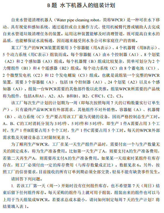
1. The topic
2. Problem Analysis
3. Model Assumptions
1. Sufficient materials for assembling small components.
2. During the production process, the production will not be interrupted due to unexpected situations such as factory power outages and mechanical failures.
3. The factory's capital flow is normal, and production will not be affected due to lack of capital.
4. Only the final product robot has external demand, and other components are not sold externally.
5. The demand for robots is determined according to the plan and is not affected by market price fluctuations.
4. Symbol description
| symbol | illustrate | unit |
|---|---|---|
| d | days | sky |
| MA1 d , MA2 d , MA3 d … MC3 d | Widget assembly quantity on day d | indivual |
| SA1 d , SA2 d , SA3 d … SC3 d | Remaining quantity of widget on day d | indivual |
| MAd , MBd ,MCd | Quantity of assembly of large components on day d | indivual |
| SAd , SBd ,SCd | Remaining quantity of large components on day d | indivual |
| DW d | The number of robots demanded on day d | indivual |
| MWd | The number of robots assembled on day d | indivual |
| SWd | The remaining number of robots on day d | indivual |
| Td | Total working hours limit on day d | working hours |
| RA1,RA2,…RB,RC | per-unit storage cost for the component | Yuan |
| FA1,FA2,…,FB,FC | Production preparation cost of the component | Yuan |
| XW d | 0-1 variable of whether to produce robots on day d | - |
| Rd | Inventory cost on day d | Yuan |
| Fd | Production preparation cost on day d | Yuan |
| checkDate t | Date of the t-th overhaul | sky |
| Tbig d | Total working hours limit on day d | working hours |
| DWpredict d | The number of robots demanded on the dth day of a week in the future | indivual |
5. Establishment and solution of problem 1 model
5.1 The establishment of the problem-model
5.1.1 Small components assemble large components
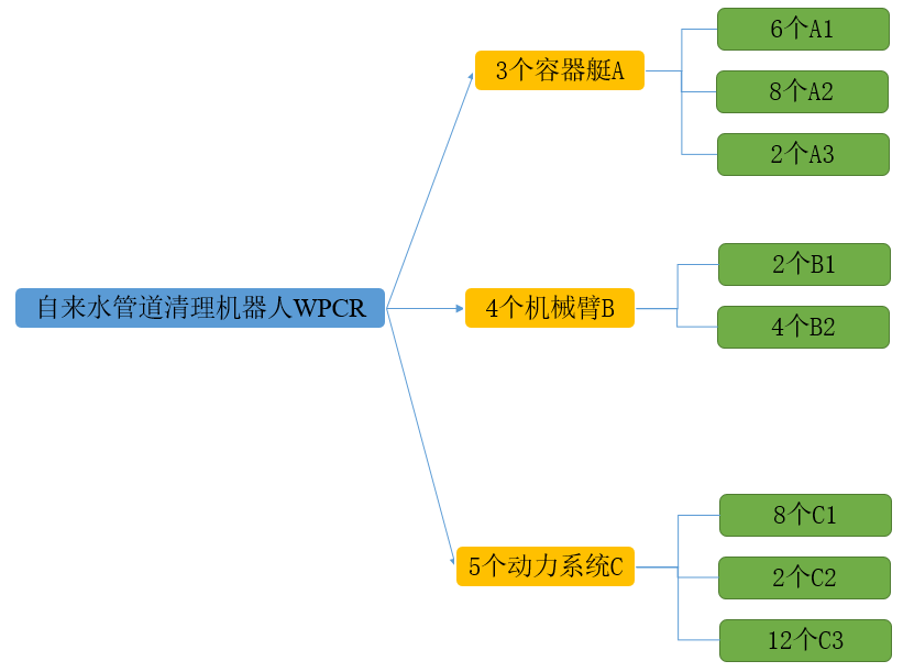
Here, the assembly of large component A is taken as an example. Assembling a large component A requires 6 small components A1, 8 small components A2, and 2 small components A3.
On day d, the number of small components A1 used to assemble the large component A is: the number of small components assembled on day d (the current day) MA1 d and the number of small components remaining on day d-1 (yesterday) SA1 d-1 and, namely MA1 d +SA1 d-1 . The number of widgets A2 and A3 can be obtained in the same way.
Assembling a large component A requires 6 small components A1. If only A1 is considered, the maximum number of large components that can be assembled is:
[ M A 1 d + S A 1 d − 1 6 ] (1) \left[ \begin{matrix} \frac{MA1_d+SA1_{d-1}}{6} \end{matrix} \right] \tag{1} [6M A 1d+ S A 1d−1]( 1 )
Note: The symbol [ ] here is rounded down, that is, take the largest integer smaller than itself.
Similarly, if only A2 is considered, the maximum number of large components A that can be assembled is:
[ M A 2 d + S A 2 d − 1 8 ] (2) \left[ \begin{matrix} \frac{MA2_d+SA2_{d-1}}{8} \end{matrix} \right] \tag{2} [8M A 2d+ S A 2d−1]( 2 )
If only A3 is considered, the maximum number of large components A that can be assembled is:
[ M A 3 d + S A 3 d − 1 2 ] (3) \left[ \begin{matrix} \frac{MA3_d+SA3_{d-1}}{2} \end{matrix} \right] \tag{3} [2M A 3d+ S A 3d−1]( 3 )
Therefore, the maximum number of assemblies of large component A on day d is:
m i n [ ( M A 1 d + S A 1 d − 1 6 , M A 2 d + S A 2 d − 1 8 , M A 3 d + S A 3 d − 1 2 ) ] (4) min\left[ \begin{pmatrix} \frac{MA1_d+SA1_{d-1}}{6}, \frac{MA2_d+SA2_{d-1}}{8}, \frac{MA3_d+SA3_{d-1}}{2} \end{pmatrix} \right]\tag{4} min[ (6M A 1d+ S A 1d−1,8M A 2d+ S A 2d−1,2M A 3d+ S A 3d−1) ]( 4 )
Note: This needs to be rounded down
The number of robots required for each day is different. To meet the demand of the order, when the factory assembles the large component A, it does not necessarily have to be equal to the maximum value. Therefore, on day d, the assembly quantity of large component A should satisfy the following constraints:
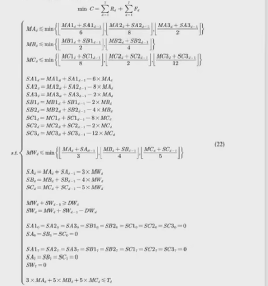
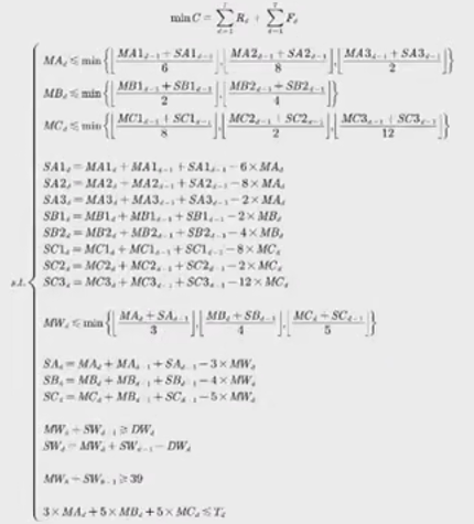
M A d ⩽ m i n [ ( M A 1 d + S A 1 d − 1 6 , M A 2 d + S A 2 d − 1 8 , M A 3 d + S A 3 d − 1 2 ) ] (5) MA_d \leqslant min\left[ \begin{pmatrix} \frac{MA1_d+SA1_{d-1}}{6}, \frac{MA2_d+SA2_{d-1}}{8}, \frac{MA3_d+SA3_{d-1}}{2} \end{pmatrix} \right]\tag{5} M Ad⩽min[ (6M A 1d+ S A 1d−1,8M A 2d+ S A 2d−1,2M A 3d+ S A 3d−1) ]( 5 )
In the same way, on the d day, the assembly quantity of large components B and C should meet the following constraints:
M B d ⩽ m i n [ ( M B 1 d + S B 1 d − 1 2 , M B 2 d + S B 2 d − 1 4 , ) ] (6) MB_d \leqslant min\left[ \begin{pmatrix} \frac{MB1_d+SB1_{d-1}}{2}, \frac{MB2_d+SB2_{d-1}}{4}, \end{pmatrix} \right]\tag{6} MBd⩽min[ (2MB 1d+SB1d−1,4MB2d+SB2d−1,) ]( 6 )
M C d ⩽ m i n [ ( M C 1 d + S C 1 d − 1 8 , M C 2 d + S C 2 d − 1 2 , M C 2 d + S C 2 d − 1 12 ) ] (6) MC_d \leqslant min\left[ \begin{pmatrix} \frac{MC1_d+SC1_{d-1}}{8}, \frac{MC2_d+SC2_{d-1}}{2}, \frac{MC2_d+SC2_{d-1}}{12} \end{pmatrix} \right]\tag{6} MCd⩽min[ (8MC 1d+ SC 1d−1,2MC 2d+SC2d−1,12MC 2d+SC2d−1) ]( 6 )
5.1.2 Remaining widgets
After assembling a large component with a small component, there may be leftovers from the small component. Here, widget A1 is used as an example.
On day d, the remaining number of widgets A1, shall satisfy, the sum of the number of widgets assembled on day d MA1 d , and the number of widgets remaining on day d-1 SA1 d-1 , minus the sum of the number of widgets on day d d-1 The consumption of Al. To assemble a large component A, 6 small components A1 are required. Therefore, the consumption amount of Al on day d is 6×MA d . Therefore, the remaining quantity SA1 d of A1 on day d is as follows:
S A 1 d = M A 1 d + S A 1 d − 1 − 6 ∗ M A d (7) SA1_d=MA1_d+SA1_{d-1} -6*MA_d \tag{7} S A 1d=M A 1d+S A 1d−1−6∗M Ad( 7 )
Today's - Consumed = Remaining
(Today's Assembled + Yesterday's Leftover) - Consumed = Remaining
The remaining number of other small components can be obtained in the same way:
SA 2 d = MA 2 d + SA 2 d − 1 − 8 ∗ MA d SA2_d=MA2_d+SA2_{d-1} -8*MA_dS A 2d=M A 2d+S A 2d−1−8∗M Ad
S A 3 d = M A 3 d + S A 3 d − 1 − 2 ∗ M A d SA3_d=MA3_d+SA3_{d-1} -2*MA_d S A 3d=M A 3d+S A 3d−1−2∗M Ad
S B 1 d = M B 1 d + S B 1 d − 1 − 2 ∗ M B d SB1_d=MB1_d+SB1_{d-1} -2*MB_d SB1d=MB 1d+SB1d−1−2∗MBd
S B 2 d = M A 1 d + S A 1 d − 1 − 4 ∗ M B d (8) SB2_d=MA1_d+SA1_{d-1} -4*MB_d \tag{8} SB2d=M A 1d+S A 1d−1−4∗MBd(8)
S C 1 d = M C 1 d + S C 1 d − 1 − 8 ∗ M C d SC1_d=MC1_d+SC1_{d-1} -8*MC_d SC 1d=MC 1d+SC 1d−1−8∗MCd
S C 2 d = M C 2 d + S C 2 d − 1 − 2 ∗ M C d SC2_d=MC2_d+SC2_{d-1} -2*MC_d SC2d=MC 2d+SC2d−1−2∗MCd
S C 3 d = M C 3 d + S C 3 d − 1 − 12 ∗ M C d SC3_d=MC3_d+SC3_{d-1} -12*MC_d SC3d=MC 3d+SC3d−1−12∗MCd
5.1.3 Calculation of the remaining large components by the assembly quantity of the robot
The assembly of the robot, that is, assembling the robot with large components, is the same as assembling large components with small components. Therefore, the number of robots assembled on the d day is as follows:
M W d ⩽ m i n [ ( M A 1 d + S A 1 d − 1 3 , M B 2 d + S B 2 d − 1 4 , M C 2 d + S C 2 d − 1 5 ) ] (9) MW_d \leqslant min\left[ \begin{pmatrix} \frac{MA1_d+SA1_{d-1}}{3}, \frac{MB2_d+SB2_{d-1}}{4}, \frac{MC2_d+SC2_{d-1}}{5} \end{pmatrix} \right]\tag{9} MWd⩽min[ (3M A 1d+ S A 1d−1,4MB2d+SB2d−1,5MC 2d+SC2d−1) ]( 9 )
Among them, MW d is the number of robots assembled, MA d is the assembly number of large components A on day d, and SA d-1 is the remaining number of large components A on day d-1.
Assemble the robot from large components, which may have some leftovers. It is calculated in the same way as calculating the remaining number of widgets, as follows:
SA d = MA d + SA d − 1 − 3 ∗ MW d SA_d=MA_d+SA_{d-1} -3*MW_dS Ad=M Ad+S Ad−1−3∗MWd
S B d = M B d + S B d − 1 − 4 ∗ M W d (10) SB_d=MB_d+SB_{d-1} -4*MW_d \tag{10} SBd=MBd+SBd−1−4∗MWd(10)
S C d = M C d + S C d − 1 − 5 ∗ M W d SC_d=MC_d+SC_{d-1} -5*MW_d SCd=MCd+SCd−1−5∗MWd
5.1.4 Robot assembly quantity constraints
All orders for robots accepted by the factory must be delivered when they expire. Therefore, the sum of the assembly quantity MW d of robots on day d and the remaining quantity SW d of robots on day d-1 should be greater than the demand quantity DW d on day d .
MW d + SW d − 1 ⩾ DW d (12) MW_d+SW_{d-1} \geqslant DW_d \tag{12}MWd+SWd−1⩾DWd( 12 )
5.1.5 Robot Remaining
There may be some leftovers after the daily sale of bots to order. The remaining SW d of the robot on the d day is equal to the sum of the assembly quantity MW d on the d day and the remaining quantity SW d-1 on the d-1 day minus the order quantity DW d on the day . which is
S W d = M W d + S W d − 1 − D W d (12) SW_d=MW_d+SW_{d-1} -DW_d \tag{12} SWd=MWd+SWd−1−DWd( 12 )
5.1.6 No Stock No Remaining
Day 1 begins without any components in stock, ie:
SA 1 0 = SA 2 0 = SA 3 0 = SB 1 0 = SB 2 0 = SC 1 0 = SC 2 0 = SC 3 0 (13) SA1_0=SA2_0= SA3_0=SB1_0=SB2_0=SC1_0=SC2_0=SC3_0 \tag{13}S A 10=S A 20=S A 30=SB10=SB20=SC 10=SC20=SC30( 13 )
SA 0 = SB 0 = SC 0 = 0 (13) SA_0=SB_0=SC_0=0 \tag{13}S A0=SB0=SC0=0( 13 )
No component inventory will be left after the seventh day, i.e.
S A 1 7 = S A 2 7 = S A 3 7 = S B 1 7 = S B 2 7 = S C 1 7 = S C 2 7 = S C 3 7 SA1_7=SA2_7=SA3_7=SB1_7=SB2_7=SC1_7=SC2_7=SC3_7 S A 17=S A 27=S A 37=SB17=SB27=SC 17=SC27=SC37
SA 7 = SB 7 = SC 7 = 0 (14) SA_7=SB_7=SC_7=0 \tag{14}S A7=SB7=SC7=0(14)
S W 7 = 0 SW_7=0 SW7=0
5.1.7 Restrictions on working hours
It takes 3 working hours to produce 1 piece of A, 5 working hours to produce 1 piece of B, and 5 working hours to produce 1 piece of C. The following constraints need to be met at one time:
3 × M A d + 5 × M B d + 5 × M C d ⩽ T d (15) 3\times MA_d+5\times MB_d+5\times MC_d \leqslant T_d \tag{15} 3×M Ad+5×MBd+5×MCd⩽Td( 15 )
5.1.8 Inventory Fee
When a component is in stock at the end of a day, the factory must pay a certain inventory fee, which is proportional to the remaining quantity of the component. Therefore, according to the remaining quantity of components on the d day, the inventory cost of small components, large components and robots can be expressed.
R s m a l l A d = R A 1 × S A 1 d + R A 2 × S A 2 d + R A 3 × S A 3 d RsmallA_d =RA1\times SA1_d+RA2\times SA2_d+RA3\times SA3_d RsmallAd=R A 1×S A 1d+R A 2×S A 2d+R A 3×S A 3d
R s m a l l B d = R B 1 × S B 1 d + R B 2 × S B 2 d RsmallB_d =RB1\times SB1_d+RB2\times SB2_d R s ma ll Bd=RB 1×SB1d+RB2×SB2d
R s m a l l C d = R C 1 × S C 1 d + R C 2 × S C 2 d + R C 3 × S C 3 d (16) RsmallC_d =RC1\times SC1_d+RC2\times SC2_d+RC3\times SC3_d \tag{16} RsmallCd=RC 1×SC 1d+RC2×SC2d+RC3×SC3d( 16 )
R b i g d = R A × S A d + R B × S B d + R C × S C d Rbig_d =RA\times SA_d+RB\times SB_d+RC\times SC_d R bi gd=R A×S Ad+RB×SBd+RC×SCd
Among them, RA1 is the single-piece inventory cost of large component A, and SA1 d is the remaining quantity of large component A on the d day. Other symbols are the same. RsmallA d , RsmallB d , and RsmallC d are the inventory costs of small components A, B, and C on the d day, Rsmall the inventory costs of the large component on the d day, and R d is the total inventory cost of the d day.
The sum is the inventory cost on day d:
R d = R s m a l l A d + R s m a l l B d + R s m a l l C d + R b i g d + R W × S W d (17) R_d =RsmallA_d+RsmallB_d+RsmallC_d+Rbig_d+RW\times SW_d \tag{17} Rd=RsmallAd+R s ma ll Bd+RsmallCd+R bi gd+RW×SWd( 17 )
5.1.9 Production preparation costs
When a factory produces a component product, it needs to pay a fixed cost that is independent of the production quantity, called the production preparation cost. In order to facilitate the calculation of the fixed cost, a 0-1 variable is introduced here. Take the 0-1 variable XW d of a production robot as an example. If a robot is produced on the d day, then XW d is 1; if no robot is produced on the d day, then XW d is 0. As follows
X W d = { 1 M W d > 0 0 M W d = 0 (18) XW_d=\begin{cases} 1 & MW_d>0 \\ 0 & MW_d=0 \\ \end{cases}\tag{18} XWd={ 10MWd>0MWd=0( 18 )
The 0-1 variables of other components can be obtained in the same way.
Therefore, according to the 0-1 variables of all components, the production preparation cost of small components, large components and robots can be expressed.
F s m a l l A d = X A 1 d × F A 1 + X A 2 d × F A 2 + X A 3 d × F A 3 FsmallA_d =XA1_d \times FA1+XA2_d \times FA2+XA3_d \times FA3 F s ma ll Ad=X A 1d×F A 1+X A 2d×F A 2+X A 3d×F A 3
F s m a l l B d = X B 1 d × F B 1 + X B 2 d × F B 2 FsmallB_d =XB1_d \times FB1+XB2_d \times FB2 FsmallBd=XB 1d×FB1+XB2d×FB2
F s m a l l C d = X C 1 d × F C 1 + X C 2 d × F C 2 + X C 3 d × F C 3 (19) FsmallC_d =XC1_d \times FC1+XC2_d \times FC2+XC3_d \times FC3 \tag{19} FsmallCd=XC 1d×FC 1+XC2d×FC 2+XC 3d×FC 3( 19 )
F b i g d = F A × X A d + F B × X B d + F C × X C d Fbig_d =FA\times XA_d+FB\times XB_d+FC\times XC_d Fbigd=F A×X Ad+FB×XBd+FC×XCd
Among them, XA1 d is the 0-1 variable of whether to produce Al on the d day, and FA1 is the production preparation cost of Al.
Other symbols are the same. FsmallA d , FsmallB d , and FsmallC d are the production preparation costs of small components A, B, and C on the d day, and the inventory cost of Fbig large components on the d day. F d is the production preparation cost on the d day.
The sum is the production preparation cost on day d:
F d = F small A d + F small B d + F small C d + F bigd + XW d × FW (20) F_d =FsmallA_d+FsmallB_d+FsmallC_d+Fbig_d+ XW_d\times FW \tag{20}Fd=F s ma ll Ad+FsmallBd+FsmallCd+Fbigd+XWd×FW( 20 )
5.1.10 Objective function
The total cost is required to be the smallest, that is, the sum of the inventory cost and the production preparation cost is the smallest, and the objective function can be obtained:
m i n C = ∑ d = 1 7 R d + ∑ d = 1 7 F d (21) min C=\sum_{d=1}^7R_d+\sum_{d=1}^7 F_d \tag{21} min C=d=1∑7Rd+d=1∑7Fd( 21 )
5.2 Problem-solving the model
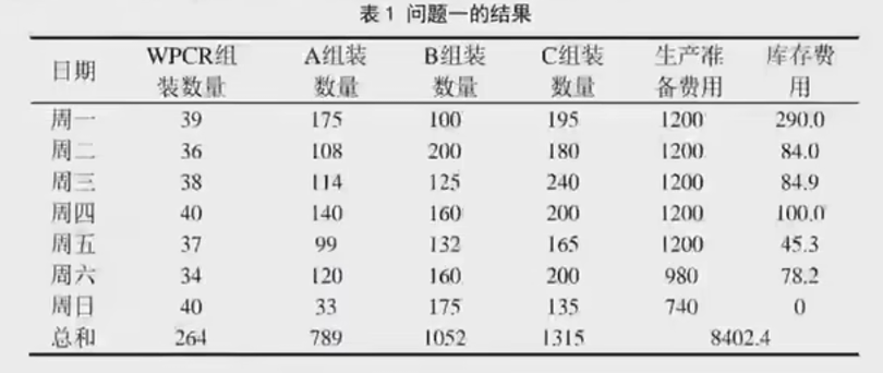
The simulated annealing algorithm is combined with the particle swarm algorithm, and the code is written in MATLAB to obtain the result of problem one, as shown below.
The result here is a bit problematic, it should be 7000+.
function [X,F]=chushihua1(WPCR,A_x,B_x,C_x,T,TA,TB,TC,W,C)
%初始化变量、计算目标函数值
flag1=0;
while flag1==0
X=[];
flag1=1;
KC_WPCR=zeros(1,length(WPCR));%记录每天WPCR库存
KC=zeros(3,length(WPCR));%记录每天ABC库存
SY_WPCR=zeros(1,length(WPCR));%记录每天交付WPCR情况
SY=zeros(3,length(WPCR));%记录每天使用ABC情况
SC_WPCR=zeros(1,length(WPCR));%记录每天组装WPCR情况
SC=zeros(3,length(WPCR));%记录每天生产ABC情况
for i=1:length(WPCR)%循环遍历每个WPCR
    if i==1%第一天0库存
        sub=[A_x,B_x,C_x].*WPCR(i);%求出每天的最小ABC需求量
        up=[];
        up(1)=fix((T(i)-sub([2,3])*[TB;TC])/TA);%BC最低供应时,A最大供应量
        up(2)=fix((T(i)-sub([1,3])*[TA;TC])/TB);%AC最低供应时,B最大供应量
        up(3)=fix((T(i)-sub([1,2])*[TA;TB])/TC);%AC最低供应时,B最大供应量
        up=min(up,fix(T(i)./([A_x,B_x,C_x]*[TA;TB;TC])).*[A_x,B_x,C_x]);
    else
        sub=max([A_x,B_x,C_x].*WPCR(i)-KC(:,i-1)',0);%除了第一天,每天减去前一天的库存则为当天至少增加的需求量
        up=[];
        up(1)=fix((T(i)-sub([2,3])*[TB;TC])/TA);%BC最低供应时,A最大供应量
        up(2)=fix((T(i)-sub([1,3])*[TA;TC])/TB);%AC最低供应时,B最大供应量
        up(3)=fix((T(i)-sub([1,2])*[TA;TB])/TC);%AC最低供应时,B最大供应量
        up=min(up,fix(T(i)./([A_x,B_x,C_x]*[TA;TB;TC])).*[A_x,B_x,C_x]);
    end
    %前面的变量会影响后面的变量范围,可能会出现上up小于sub的情况,毕竟有最大工时限制
    if length(find((up-sub)<0))>0%如果出现则重新生成
        flag1=0;
        continue
    end
    flag2=0;
    while flag2==0
        x=[randi([sub(1),up(1)]),randi([sub(2),up(2)]),randi([sub(3),up(3)])];%在区间内随机生成整数
        if x*[TA;TB;TC]<=T(i)%需求量必须满足在工时限制内
            flag2=1;
        end
    end
    %每天组装的WPCR
    if i==1
        s=WPCR(i);%可组装最小数量
        u=min(fix(x./[A_x,B_x,C_x]));%可组装最大数量
    else
        s=WPCR(i)-KC_WPCR(i-1);
        u=min(fix([x+KC(:,i-1)']./[A_x,B_x,C_x]));
    end
    %更新SC、KC、SY矩阵
    %生产
    SC_WPCR(i)=randi([s,u]);
    SC(:,i)=SC(:,i)+x';
    %放库存
    if i==1
        KC_WPCR(i)=KC_WPCR(i)+SC_WPCR(i);
        KC(:,i)=KC(:,i)+SC(:,i);
    else
        KC_WPCR(i)=KC_WPCR(i-1)+SC_WPCR(i);
        KC(:,i)=KC(:,i-1)+SC(:,i);
    end
    %使用
    SY_WPCR(i)=WPCR(i);
    SY(:,i)=[A_x;B_x;C_x].*SC_WPCR(i);
    %更新库存
    KC_WPCR(i)=KC_WPCR(i)-WPCR(i);
    KC(:,i)=KC(:,i)-SY(:,i);
end
X=[SC_WPCR;SC];
X=reshape(X',1,28);
end
X1=[SC_WPCR;SC];%生产
X2=[KC_WPCR;KC];%库存
X1(find(X1>0))=1;
%最优情况,小件无库存但是有生产准备费用
f1=sum(X1.*[W(1);sum(W(2:5));sum(W(6:8));sum(W(9:12))],2);
f2=sum(X2.*C([1,2,6,9])',2);
F=sum(f1)+sum(f2);"
function J=jianyan1(X,WPCR,A_x,B_x,C_x)
%检验变量参与运算后是否出现小于0的值,是则不满足条件
X=X';
KC_WPCR=zeros(1,length(WPCR));%记录每天WPCR库存
KC=zeros(3,length(WPCR));%记录每天ABC库存
SY_WPCR=zeros(1,length(WPCR));%记录每天交付WPCR情况
SY=zeros(3,length(WPCR));%记录每天使用ABC情况
SC_WPCR=zeros(1,length(WPCR));%记录每天组装WPCR情况
SC=zeros(3,length(WPCR));%记录每天生产ABC情况
for i=1:length(WPCR)%循环遍历每个WPCR
    x=X(i,2:4);
    %更新SC、KC、SY矩阵
    %生产
    SC_WPCR(i)=X(i,1);
    SC(:,i)=SC(:,i)+x';
    %放库存
    if i==1
        KC_WPCR(i)=KC_WPCR(i)+SC_WPCR(i);
        KC(:,i)=KC(:,i)+SC(:,i);
    else
        KC_WPCR(i)=KC_WPCR(i-1)+SC_WPCR(i);
        KC(:,i)=KC(:,i-1)+SC(:,i);
    end
    %使用
    SY_WPCR(i)=WPCR(i);
    SY(:,i)=[A_x;B_x;C_x].*SC_WPCR(i);
    %更新库存
    KC_WPCR(i)=KC_WPCR(i)-WPCR(i);
    KC(:,i)=KC(:,i)-SY(:,i);
end
if length(find(KC_WPCR<0))>0 | length(find(KC<0))>0
    J=1;
else
    J=0;
end
function [F,f1,f2]=fun1(X,WPCR,A_x,B_x,C_x,W,C)
%带入变量计算目标函数值
X=reshape(X',7,4);
KC_WPCR=zeros(1,length(WPCR));%记录每天WPCR库存
KC=zeros(3,length(WPCR));%记录每天ABC库存
SY_WPCR=zeros(1,length(WPCR));%记录每天交付WPCR情况
SY=zeros(3,length(WPCR));%记录每天使用ABC情况
SC_WPCR=zeros(1,length(WPCR));%记录每天组装WPCR情况
SC=zeros(3,length(WPCR));%记录每天生产ABC情况
for i=1:length(WPCR)%循环遍历每个WPCR
    x=X(i,2:4);
    %更新SC、KC、SY矩阵
    %生产
    SC_WPCR(i)=X(i,1);
    SC(:,i)=SC(:,i)+x';
    %放库存
    if i==1
        KC_WPCR(i)=KC_WPCR(i)+SC_WPCR(i);
        KC(:,i)=KC(:,i)+SC(:,i);
    else
        KC_WPCR(i)=KC_WPCR(i-1)+SC_WPCR(i);
        KC(:,i)=KC(:,i-1)+SC(:,i);
    end
    %使用
    SY_WPCR(i)=WPCR(i);
    SY(:,i)=[A_x;B_x;C_x].*SC_WPCR(i);
    %更新库存
    KC_WPCR(i)=KC_WPCR(i)-WPCR(i);
    KC(:,i)=KC(:,i)-SY(:,i);
end
X1=[SC_WPCR;SC];%生产
X2=[KC_WPCR;KC];%库存
X1(find(X1>0))=1;
%最优情况,小件无库存但是有生产准备费用
f1=sum(X1.*[W(1);sum(W(2:5));sum(W(6:8));sum(W(9:12))],1)';
f2=sum(X2.*C([1,2,6,9])',1)';
F=sum(f1)+sum(f2);
clear all
clc
%每天WPCR需求量
WPCR=[39 36 38 40 37 33 40];
%一个WPCR队ABC需求比例
A_x=3;
B_x=4;
C_x=5;
%每天总工时
T=[4500 2500 2750 2100 2500 2750 1500];
%ABC单位工时消耗
TA=3;
TB=5;
TC=5;
%生产准备费用:A A1 A2 A3 B B1 B2 C C1 C2 C3
W=[240 120 40 60 50 160 80 100 180 60 40 70];
%单件库存费用:A A1 A2 A3 B B1 B2 C C1 C2 C3
C=[5 2 5 3 6 1.5 4 5 1.7 3 2 3];

%模拟退火-粒子群算法
T0=100; %初始化温度值
T_min=1; %设置温度下界
alpha=0.95; %温度的下降率
c1=0.4;c2=0.6; %学习因子
wmax=0.6;wmin=0.4; %惯性权重
num=1000; %颗粒总数,效果不好可以增加
X=[];
F=[];
for i=1:num
    [X(i,:),F(i,1)]=chushihua1(WPCR,A_x,B_x,C_x,T,TA,TB,TC,W,C);
end
%以最小化为例
[bestf,a]=min(F);
bestx=X(a,:);
trace(1)=bestf;
while(T0>T_min)
    XX=[];
    FF=[];
 for i=1:num
        [XX(i,:),FF(i,1)]=chushihua1(WPCR,A_x,B_x,C_x,T,TA,TB,TC,W,C);
        delta=FF(i,1)-F(i,1);
        if delta<0
            F(i,1)=FF(i,1);
            X(i,:)=XX(i,:);
        else
            P=exp(-delta/T0);
            if P>rand
                F(i,1)=FF(i,1);
                X(i,:)=XX(i,:);
            end
        end
    end
    fave=mean(F);
    fmin=min(F);
    for i=1:num
        %权重更新
        if F(i)<=fave
            w=wmin+(F(i)-fmin)*(wmax-wmin)/(fave-fmin);
        else
            w=wmax;
        end
        [~,b]=min(F);
        best=X(b,:);%当前最优解
        v=w.*randn(1,28)+c1*rand*(best-X(i,:))+c2*rand*(bestx-X(i,:));%速度
        XX(i,:)=round(X(i,:)+v);%更新位置
        XX(i,:)=max(XX(i,:),0);%不能小于0
        %检验,不满足条件则返回之前的变量
        x=reshape(XX(i,:)',7,4)';%重新排列矩阵维度
        J=jianyan1(X,WPCR,A_x,B_x,C_x);
        if length(find((sum(x(2:4,:).*[TA;TB;TC],1)-T)>0))>0 | sum(x(1,:))<sum(WPCR) | J==1
            XX(i,:)=X(i,:);
        end
        %计算目标函数
        FF(i,1)=fun1(X(i,:),WPCR,A_x,B_x,C_x,W,C);
        %更新最优
        if FF(i,1)<F(i,1)
            F(i,1)=FF(i,1);
            X(i,:)=XX(i,:);
        end
    end
    if min(F)<bestf
        [bestf,a]=min(F);
        bestx=X(a,:);
    end
    trace=[trace;bestf];
    T0=T0*alpha;
end
disp('最优解为:')
disp('WPCR组装数量、A组装数量、B组装数量、C组装数量')
disp(reshape(bestx',7,4))
disp('生产准备费用、库存费用')
[~,f1,f2]=fun1(bestx,WPCR,A_x,B_x,C_x,W,C)
disp('总费用')
disp(bestf)
figure
plot(trace)
xlabel('迭代次数')
ylabel('函数值')
title('模拟退火算法')
legend('最优值')
6. Resume and solution of problem 2 model
6.1 Establishment of the second problem model
6.1.1 Small components assemble large components
Components A, B, and C need to be produced and put into storage one day in advance to assemble WPCR, and components A1, A2, A3, B1, B2, C1, C2, and C3 also need to be produced and put into storage one day in advance to assemble A, B, and C. Therefore, if you want to complete the order demand for components on Monday, you need to assemble the large components A, B, and C required on Monday last week on Sunday. And last Sunday, the small components used to assemble the large components should be assembled on the last Saturday.
Therefore, the number of small components used to assemble large components on day d should be the sum of the number of small components assembled on day d-1 and the number of small components remaining on day d-1. Therefore, formulas (5) and (6) are modified to obtain the constraints of large components, as follows:
MA d ⩽ min [ ( MA 1 d − 1 + SA 1 d − 1 6 , MA 2 d − 1 + SA 2 d − 1 8 , MA 3 d − 1 + SA 3 d − 1 2 ) ] MA_d \leqslant min\left[ \begin{pmatrix} \frac{MA1_{d-1}+SA1_{d-1}}{6 }, \frac{MA2_{d-1}+SA2_{d-1}}{8}, \frac{MA3_{d-1}+SA3_{d-1}}{2} \end{pmatrix} \right ]M Ad⩽min[ (6M A 1d−1+ S A 1d−1,8M A 2d−1+ S A 2d−1,2M A 3d−1+ S A 3d−1) ]
M B d ⩽ m i n [ ( M B 1 d − 1 + S B 1 d − 1 2 , M B 2 d − 1 + S B 2 d − 1 4 , ) ] (22) MB_d \leqslant min\left[ \begin{pmatrix} \frac{MB1_{d-1}+SB1_{d-1}}{2}, \frac{MB2_{d-1}+SB2_{d-1}}{4}, \end{pmatrix} \right]\tag{22} MBd⩽min[ (2MB 1d−1+SB1d−1,4MB2d−1+SB2d−1,) ]( 22 )
M C d ⩽ m i n [ ( M C 1 d − 1 + S C 1 d − 1 8 , M C 2 d − 1 + S C 2 d − 1 2 , M C 3 d − 1 + S C 3 d − 1 12 ) ] MC_d \leqslant min\left[ \begin{pmatrix} \frac{MC1_{d-1}+SC1_{d-1}}{8}, \frac{MC2_{d-1}+SC2_{d-1}}{2}, \frac{MC3_{d-1}+SC3_{d-1}}{12} \end{pmatrix} \right] MCd⩽min[ (8MC 1d−1+ SC 1d−1,2MC 2d−1+SC2d−1,12MC 3d−1+SC3d−1) ]
6.1.2 Remaining widgets
The number of widgets remaining on day d, that is, the number of widgets that need to be stored, can be viewed as two parts. One part is the number of small components assembled on day d, and the other part is the remaining part of large components assembled on day d, and the remaining part should be the number of small components assembled on day d-1 and the number of remaining small components on day d-1. and, minus the amount consumed on day d,
Day d remaining { quantity assembled on day d + (quantity assembled on day d − 1 + quantity remaining on day d − 1) − quantity consumed on day d remaining on day d\begin{cases} day d Quantity Assembled\\ +\\ (Quantity Assembled on Day d-1 + Quantity Remaining on Day d-1) - Quantity Consumed on Day d\end{cases}Day d remaining⎩ ⎨ ⎧Quantity assembled on day d+(th d−Quantity assembled in 1 day+d _−1 day remaining quantity)−Quantity consumed on day d
So the rest of the widget looks like this:
S A 1 d = M A 1 d + M A 1 d − 1 + S A 1 d − 1 − 6 × M A d SA1_d=MA1_d+MA1_{d-1}+SA1_{d-1}-6 \times MA_d S A 1d=M A 1d+M A 1d−1+S A 1d−1−6×M Ad
S A 2 d = M A 2 d + M A 2 d − 1 + S A 2 d − 1 − 8 × M A d SA2_d=MA2_d+MA2_{d-1}+SA2_{d-1}-8 \times MA_d S A 2d=M A 2d+M A 2d−1+S A 2d−1−8×M Ad
S A 3 d = M A 3 d + M A 3 d − 1 + S A 3 d − 1 − 2 × M A d SA3_d=MA3_d+MA3_{d-1}+SA3_{d-1}-2 \times MA_d S A 3d=M A 3d+M A 3d−1+S A 3d−1−2×M Ad
S B 1 d = M B 1 d + M B 1 d − 1 + S B 1 d − 1 − 2 × M B d SB1_d=MB1_d+MB1_{d-1}+SB1_{d-1}-2 \times MB_d SB1d=MB 1d+MB 1d−1+SB1d−1−2×MBd
S B 2 d = M B 2 d + M B 2 d − 1 + S B 2 d − 1 − 4 × M B d (23) SB2_d=MB2_d+MB2_{d-1}+SB2_{d-1}-4 \times MB_d \tag{23} SB2d=MB2d+MB2d−1+SB2d−1−4×MBd(23)
S C 1 d = M C 1 d + M C 1 d − 1 + S C 1 d − 1 − 8 × M C d SC1_d=MC1_d+MC1_{d-1}+SC1_{d-1}-8 \times MC_d SC 1d=MC 1d+MC 1d−1+SC 1d−1−8×MCd
S C 2 d = M C 2 d + M C 2 d − 1 + S C 2 d − 1 − 2 × M C d SC2_d=MC2_d+MC2_{d-1}+SC2_{d-1}-2 \times MC_d SC2d=MC 2d+MC 2d−1+SC2d−1−2×MCd
S C 3 d = M C 3 d + M C 3 d − 1 + S C 3 d − 1 − 12 × M C d SC3_d=MC3_d+MC3_{d-1}+SC3_{d-1}-12 \times MC_d SC3d=MC 3d+MC 3d−1+SC3d−1−12×MCd
6.1.3 The assembly quantity of the robot calculates the remaining large components
The assembly of the robot is the same as the assembly of small components to large components. On day d, the robot is assembled using the assembly on day d-1 or the remaining large components. The constraints are as follows:
M W d ⩽ m i n [ ( M A 1 d − 1 + S A 1 d − 1 3 , M B 2 d − 1 + S B 2 d − 1 4 , M C 3 d − 1 + S C 3 d − 1 5 ) ] (24) MW_d \leqslant min\left[ \begin{pmatrix} \frac{MA1_{d-1}+SA1_{d-1}}{3}, \frac{MB2_{d-1}+SB2_{d-1}}{4}, \frac{MC3_{d-1}+SC3_{d-1}}{5} \end{pmatrix} \right]\tag{24} MWd⩽min[ (3M A 1d−1+ S A 1d−1,4MB2d−1+SB2d−1,5MC 3d−1+SC3d−1) ]( 24 )
The remainder of the large component is the same as the remainder of the small component, as follows:
SA d = MA d + MA d − 1 + SA d − 1 − 3 × MW d SA_d=MA_d+MA_{d-1}+SA_{d-1}-3 \times MW_dS Ad=M Ad+M Ad−1+S Ad−1−3×MWd
S B d = M B d + M B d − 1 + S B d − 1 − 4 × M W d (25) SB_d=MB_d+MB_{d-1}+SB_{d-1}-4 \times MW_d \tag{25} SBd=MBd+MBd−1+SBd−1−4×MWd(25)
S C d = M C d + M C d − 1 + S C d − 1 − 5 × M W d SC_d=MC_d+MC_{d-1}+SC_{d-1}-5 \times MW_d SCd=MCd+MCd−1+SCd−1−5×MWd
6.1.4 Robot assembly quantity constraints and residual calculation
The assembly quantity and remainder of the robot are unmodified as follows:
M W d + S W d − 1 ⩾ D W d (26) MW_d+SW_{d-1} \geqslant DW_d \tag{26} MWd+SWd−1⩾DWd(26)
S W d = M C d + M W d − 1 + S W d − 1 − D W d (26) SW_d=MC_d+MW_{d-1}+SW_{d-1}-DW_d \tag{26} SWd=MCd+MWd−1+SWd−1−DWd( 26 )
6.1.5 Guarantee the production of the next day
In order to ensure the production on Monday next week, the components should be left at the end of this week on Sunday, so equations (13) and (14) in question 1 should not be considered. Consider the next Monday as the 8th day, so the sum of the number of robots assembled on the 8th day and the remaining number of robots on the 7th day should not be less than the order quantity 39 on the next Monday, as follows:
M W 8 + S W 8 − 1 ⩾ 39 (26) MW_8+SW_{8-1} \geqslant 39 \tag{26} MW8+SW8 − 1⩾39( 26 )
It is worth noting that in this week, in order to ensure the production of robots on day d, the constraints on the assembly quantity of large components on day d and the assembly quantity of small components on day d-1 are not clearly given. However, in equation (26), there is a constraint on the order quantity DW d of robots on the d day and the quantity MW d manufactured on the d day . There is a constraint on the assembly quantity of large components on day d, in equation (22), there is a constraint on the assembly quantity of small components on day d-1 on the number of large components assembled on day d.
Therefore, the constraints to guarantee the number of robots produced on the second day are not explicitly given, but they are implied.
6.1.6 Restrictions on working hours
The working hours limit is not modified as follows:
3 × MA d + 5 × MB d + 5 × MC d ⩽ T d (27) 3\times MA_d+5\times MB_d+5\times MC_d \leqslant T_d \tag {27}3×M Ad+5×MBd+5×MCd⩽Td( 27 )
6.1.7 Objective function
The objective function is not modified and is the same as problem 1 as follows:
min C = ∑ d = 1 7 R d + ∑ d = 1 7 F d (28) min C=\sum_{d=1}^7R_d+\sum_ {d=1}^7 F_d \tag{28}min C=d=1∑7Rd+d=1∑7Fd( 28 )
6.2 The solution of the second problem model
Use MATLAB to write the code to obtain the result of the second question.
clear
clc
%每天WPCR需求量
WPCR=[39 36 38 40 37 33 40];
%一个WPCR队ABC需求比例
A_x=3;
B_x=4;
C_x=5;
D_x=[6;8;2;2;4;8;2;12];
%每天总工时
T=[4500 2500 2750 2100 2500 2750 1500];
%ABC单位工时消耗
TA=3;
TB=5;
TC=5;
%生产准备费用:A A1 A2 A3 B B1 B2 C C1 C2 C3
W=[240 120 40 60 50 160 80 100 180 60 40 70];
%单件库存费用:A A1 A2 A3 B B1 B2 C C1 C2 C3
C=[5 2 5 3 6 1.5 4 5 1.7 3 2 3];

%模拟退火-粒子群算法
T0=100; %初始化温度值
T_min=1; %设置温度下界
alpha=0.95; %温度的下降率
c1=0.4;c2=0.6; %学习因子
wmax=0.6;wmin=0.4; %惯性权重
num=1000; %颗粒总数
X=[];
F=[];
for i=1:num
    [X(i,:),F(i,1)]=chushihua2(WPCR,A_x,B_x,C_x,T,TA,TB,TC,W,C,D_x);
end
%以最小化为例
[bestf,a]=min(F);
bestx=X(a,:);
trace(1)=bestf;
while(T0>T_min)
    XX=[];
    FF=[];
 for i=1:num
        [XX(i,:),FF(i,1)]=chushihua2(WPCR,A_x,B_x,C_x,T,TA,TB,TC,W,C,D_x);
        delta=FF(i,1)-F(i,1);
        if delta<0
            F(i,1)=FF(i,1);
            X(i,:)=XX(i,:);
        else
            P=exp(-delta/T0);
            if P>rand
                F(i,1)=FF(i,1);
                X(i,:)=XX(i,:);
            end
        end
    end
    fave=mean(F);
    fmin=min(F);
    for i=1:num
        %权重更新
        if F(i)<=fave
            w=wmin+(F(i)-fmin)*(wmax-wmin)/(fave-fmin);
        else
            w=wmax;
        end
        [~,b]=min(F);
        best=X(b,:);%当前最优解
        v=w.*randn(1,28)+c1*rand*(best-X(i,:))+c2*rand*(bestx-X(i,:));%速度
        XX(i,:)=round(X(i,:)+v);%更新位置
        XX(i,:)=max(XX(i,:),0);%不能小于0
        %检验,不满足条件则返回之前的变量
        x=reshape(XX(i,:)',7,4)';%重新排列矩阵维度
        J=jianyan2(X,WPCR,A_x,B_x,C_x,D_x);
        if length(find((sum(x(2:4,:).*[TA;TB;TC],1)-T)>0))>0 | sum(x(1,:))<sum(WPCR) | J==1
            XX(i,:)=X(i,:);
        end
        %计算目标函数
        FF(i,1)=fun2(X(i,:),WPCR,A_x,B_x,C_x,W,C,D_x);
        %更新最优
        if FF(i,1)<F(i,1)
            F(i,1)=FF(i,1);
            X(i,:)=XX(i,:);
        end
    end
    if min(F)<bestf
        [bestf,a]=min(F);
        bestx=X(a,:);
    end
    trace=[trace;bestf];
    T0=T0*alpha;
end
disp('最优解为:')
disp('WPCR组装数量、A组装数量、B组装数量、C组装数量')
disp(reshape(bestx',7,4))
disp('生产准备费用、库存费用')
[~,f1,f2]=fun2(bestx,WPCR,A_x,B_x,C_x,W,C,D_x)
disp('总费用')
disp(bestf)
figure
plot(trace)
xlabel('迭代次数')
ylabel('函数值')
title('模拟退火算法')
legend('最优值')
function [X,F]=chushihua2(WPCR,A_x,B_x,C_x,T,TA,TB,TC,W,C,D_x)
%初始化变量、计算目标函数值,小件提前两天,大件提前1天
flag1=0;
while flag1==0
X=[];
nn=2;%延迟天数
flag1=1;
KC_WPCR=zeros(1,length(WPCR)+nn);%记录每天WPCR库存
KC=zeros(3,length(WPCR)+nn);%记录每天ABC库存
KC_x=zeros(8,length(WPCR)+nn);%记录每天ABC小件库存
SY_WPCR=zeros(1,length(WPCR)+nn);%记录每天交付WPCR情况
SY=zeros(3,length(WPCR)+nn);%记录每天使用ABC情况
SY_x=zeros(8,length(WPCR)+nn);%记录每天使用ABC小件情况
SC_WPCR=zeros(1,length(WPCR)+nn);%记录每天组装WPCR情况
SC=zeros(3,length(WPCR)+nn);%记录每天生产ABC情况
SC_x=zeros(8,length(WPCR)+nn);%记录每天生产ABC小件情况
for i=1:length(WPCR)%循环遍历每个WPCR
    if i==1%假设第一天刚好满足WPCR
        sub=[A_x,B_x,C_x].*WPCR(i);%求出每天的WPCR最小ABC需求量
        up=sub;
    else
        sub=max([A_x,B_x,C_x].*WPCR(i)-KC(:,i+nn-1)',0);%除了第一天,每天减去前一天的库存则为当天至少增加的需求量
        up=[];
        up(1)=fix((T(i)-sub([2,3])*[TB;TC])/TA);%BC最低供应时,A最大供应量
        up(2)=fix((T(i)-sub([1,3])*[TA;TC])/TB);%AC最低供应时,B最大供应量
        up(3)=fix((T(i)-sub([1,2])*[TA;TB])/TC);%AC最低供应时,B最大供应量
        up=min(up,fix(T(i)./([A_x,B_x,C_x]*[TA;TB;TC])).*[A_x,B_x,C_x]);
    end
    %前面的变量会影响后面的变量范围,可能会出现上up小于sub的情况,毕竟有最大工时限制
    if length(find((up-sub)<0))>0%如果出现则重新生成
        flag1=0;
        continue
    end
    flag2=0;
    while flag2==0
        x=[randi([sub(1),up(1)]),randi([sub(2),up(2)]),randi([sub(3),up(3)])];%在区间内随机生成整数
        if x*[TA;TB;TC]<=T(i)%需求量必须满足在工时限制内
            flag2=1;
        end
    end
    %每天组装的WPCR
    if i==1
        s=WPCR(i);%可组装最小数量
        u=min(fix(x./[A_x,B_x,C_x]));%可组装最大数量
    else
        s=WPCR(i)-KC_WPCR(i+nn-1);
        u=min(fix([x+KC(:,i+nn-1)']./[A_x,B_x,C_x]));
    end
    %更新SC、KC、SY矩阵
    %生产
    SC_WPCR(i+nn)=randi([s,u]);
    SC(:,i+nn-1)=SC(:,i+nn-1)+x';
    SC_x(1:3,i)=D_x(1:3).*SC(1,i+nn-1);
    SC_x(4:5,i)=D_x(4:5).*SC(2,i+nn-1);
    SC_x(6:8,i)=D_x(6:8).*SC(3,i+nn-1);
    %放库存
    KC_WPCR(i+nn)=KC_WPCR(i+nn-1)+SC_WPCR(i+nn);
    KC(:,i+nn-1)=KC(:,i+nn-2)+SC(:,i+nn-1);
    if i==1
       KC_x(:,i+nn-2)=SC_x(:,i+nn-2);
    else
       KC_x(:,i+nn-2)=KC_x(:,i+nn-3)+SC_x(:,i+nn-2);
    end
    %使用
    SY_WPCR(i+nn)=WPCR(i);
    SY(:,i+nn)=[A_x;B_x;C_x].*SY_WPCR(i+nn);
    SY_x(1:3,i+nn-1)=D_x(1:3).*SY(1,i+nn);
    SY_x(4:5,i+nn-1)=D_x(4:5).*SY(2,i+nn);
    SY_x(6:8,i+nn-1)=D_x(6:8).*SY(3,i+nn);
    %更新库存
    KC_WPCR(i+nn)=KC_WPCR(i+nn)-WPCR(i);
    KC(:,i+nn)=KC(:,i+nn-1)-SY(:,i+nn);
    KC_x(:,i+nn-1)=KC_x(:,i+nn-2)-SY_x(:,i+nn-1);
end
X=[SC_WPCR(:,nn+1:end);SC(:,nn:end-1)];
X=reshape(X',1,28);
end
X1=[SC_WPCR(:,nn+1:end);SC(:,nn+1:end)];%生产
X2=[SC_x(:,nn+1:end)];%生产ABC小件
X3=[KC_WPCR(:,nn+1:end);KC(:,nn+1:end)];%库存ABC
X4=[KC_x(:,nn+1:end)];%库存ABC小件
X1(find(X1>0))=1;
X2(find(X2>0))=1;
%最优情况,小件无库存但是有生产准备费用
f1=(sum(X1.*[W(1);W(2);W(6);W(9)],1)+sum(X2.*[W(3:5)';W(7:8)';W(10:12)'],1))';
f2=(sum(X3.*C([1,2,6,9])',1)+sum(X4.*C([3,4,5,7,8,10,11,12])',1))';
F=sum(f1)+sum(f2);
function [F,f1,f2]=fun2(X,WPCR,A_x,B_x,C_x,W,C,D_x)
%初始化变量、计算目标函数值
X=reshape(X',7,4);
nn=2;
KC_WPCR=zeros(1,length(WPCR)+nn);%记录每天WPCR库存
KC=zeros(3,length(WPCR)+nn);%记录每天ABC库存
KC_x=zeros(8,length(WPCR)+nn);%记录每天ABC小件库存
SY_WPCR=zeros(1,length(WPCR)+nn);%记录每天交付WPCR情况
SY=zeros(3,length(WPCR)+nn);%记录每天使用ABC情况
SY_x=zeros(8,length(WPCR)+nn);%记录每天使用ABC小件情况
SC_WPCR=zeros(1,length(WPCR)+nn);%记录每天组装WPCR情况
SC=zeros(3,length(WPCR)+nn);%记录每天生产ABC情况
SC_x=zeros(8,length(WPCR)+nn);%记录每天生产ABC小件情况
for i=1:length(WPCR)%循环遍历每个WPCR
    x=X(i,2:4);
    %更新SC、KC、SY矩阵
    %生产
    SC_WPCR(i+nn)=X(i,1);
    SC(:,i+nn-1)=SC(:,i+nn-1)+x';
    SC_x(1:3,i)=D_x(1:3).*SC(1,i+nn-1);
    SC_x(4:5,i)=D_x(4:5).*SC(2,i+nn-1);
    SC_x(6:8,i)=D_x(6:8).*SC(3,i+nn-1);
    %放库存
    KC_WPCR(i+nn)=KC_WPCR(i+nn-1)+SC_WPCR(i+nn);
    KC(:,i+nn-1)=KC(:,i+nn-2)+SC(:,i+nn-1);
    if i==1
       KC_x(:,i+nn-2)=SC_x(:,i+nn-2);
    else
       KC_x(:,i+nn-2)=KC_x(:,i+nn-3)+SC_x(:,i+nn-2);
    end
    %使用
    SY_WPCR(i+nn)=WPCR(i);
    SY(:,i+nn)=[A_x;B_x;C_x].*SY_WPCR(i+nn);
    SY_x(1:3,i+nn-1)=D_x(1:3).*SY(1,i+nn);
    SY_x(4:5,i+nn-1)=D_x(4:5).*SY(2,i+nn);
    SY_x(6:8,i+nn-1)=D_x(6:8).*SY(3,i+nn);
    %更新库存
    KC_WPCR(i+nn)=KC_WPCR(i+nn)-WPCR(i);
    KC(:,i+nn)=KC(:,i+nn-1)-SY(:,i+nn);
    KC_x(:,i+nn-1)=KC_x(:,i+nn-2)-SY_x(:,i+nn-1);
end
X1=[SC_WPCR(:,nn+1:end);SC(:,nn+1:end)];%生产
X2=[SC_x(:,nn+1:end)];%生产ABC小件
X3=[KC_WPCR(:,nn+1:end);KC(:,nn+1:end)];%库存ABC
X4=[KC_x(:,nn+1:end)];%库存ABC小件
X1(find(X1>0))=1;
X2(find(X2>0))=1;
%最优情况,小件无库存但是有生产准备费用
f1=(sum(X1.*[W(1);W(2);W(6);W(9)],1)+sum(X2.*[W(3:5)';W(7:8)';W(10:12)'],1))';
f2=(sum(X3.*C([1,2,6,9])',1)+sum(X4.*C([3,4,5,7,8,10,11,12])',1))';
F=sum(f1)+sum(f2);
function J=jianyan2(X,WPCR,A_x,B_x,C_x,D_x)
%检验变量参与运算后是否出现小于0的值,是则不满足条件
X=X';
nn=2;
KC_WPCR=zeros(1,length(WPCR)+nn);%记录每天WPCR库存
KC=zeros(3,length(WPCR)+nn);%记录每天ABC库存
KC_x=zeros(8,length(WPCR)+nn);%记录每天ABC小件库存
SY_WPCR=zeros(1,length(WPCR)+nn);%记录每天交付WPCR情况
SY=zeros(3,length(WPCR)+nn);%记录每天使用ABC情况
SY_x=zeros(8,length(WPCR)+nn);%记录每天使用ABC小件情况
SC_WPCR=zeros(1,length(WPCR)+nn);%记录每天组装WPCR情况
SC=zeros(3,length(WPCR)+nn);%记录每天生产ABC情况
SC_x=zeros(8,length(WPCR)+nn);%记录每天生产ABC小件情况
for i=1:length(WPCR)%循环遍历每个WPCR
    x=X(i,2:4);
    %更新SC、KC、SY矩阵
    %生产
    SC_WPCR(i+nn)=X(i,1);
    SC(:,i+nn-1)=SC(:,i+nn-1)+x';
    SC_x(1:3,i)=D_x(1:3).*SC(1,i+nn-1);
    SC_x(4:5,i)=D_x(4:5).*SC(2,i+nn-1);
    SC_x(6:8,i)=D_x(6:8).*SC(3,i+nn-1);
    %放库存
    KC_WPCR(i+nn)=KC_WPCR(i+nn-1)+SC_WPCR(i+nn);
    KC(:,i+nn-1)=KC(:,i+nn-2)+SC(:,i+nn-1);
    if i==1
       KC_x(:,i+nn-2)=SC_x(:,i+nn-2);
    else
       KC_x(:,i+nn-2)=KC_x(:,i+nn-3)+SC_x(:,i+nn-2);
    end
    %使用
    SY_WPCR(i+nn)=WPCR(i);
    SY(:,i+nn)=[A_x;B_x;C_x].*SY_WPCR(i+nn);
    SY_x(1:3,i+nn-1)=D_x(1:3).*SY(1,i+nn);
    SY_x(4:5,i+nn-1)=D_x(4:5).*SY(2,i+nn);
    SY_x(6:8,i+nn-1)=D_x(6:8).*SY(3,i+nn);
    %更新库存
    KC_WPCR(i+nn)=KC_WPCR(i+nn)-WPCR(i);
    KC(:,i+nn)=KC(:,i+nn-1)-SY(:,i+nn);
    KC_x(:,i+nn-1)=KC_x(:,i+nn-2)-SY_x(:,i+nn-1);
end
if length(find(KC_WPCR<0))>0 | length(find(KC<0))>0 | length(find(KC_x<0))>0
    J=1;
else
    J=0;
end
7. Establishment and solution of problem three model
7.1 Establishment of the third problem model
7.1.1 Determination of time variables
In this question, the time has changed from 7 days to 30 weeks and 210 days, so the time variable is
d ∈ ( − 1 , 0 , 1 , . . . , 208 , 209 , 210 ) (29) d ∈ (-1,0, 1, ..., 208, 209, 210) \tag{29}d∈(−1 ,0 , 1 , ... , 208 ,209 ,210 )( 29 )
d=-1 is the Saturday of the previous week in week 1, and d=0 is the Sunday of the previous week in week 1. d=1 is the Monday of the 1st week, which is the first day of the 30th week; d=210 is the Sunday of the 30th week, which is the last day of the 30th week.
7.1.2 0-1 variables for downtime
In modeling, when encountering the problem that a variable can take multiple integer values, a set of 0-1 variables can be used to replace the variable by taking advantage of the property that a 0-1 variable is a binary variable. Therefore, by virtue of this property, a set of 0-1 variables is introduced to replace one downtime 0-1 variable.
Taking the first maintenance date as an example, the model for the first maintenance day is established as follows:
checki = { 1 Inspection on day i 0 No inspection on day i(29) check_i=\begin{cases} 1 & Inspection on day i \\ 0 & No inspection on day i \\ \end{cases}\tag {29}checki={ 10Day i to be overhauledNo maintenance on day i( 29 )
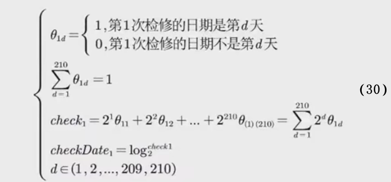
In the above formula, the first formula is a 0-1 variable, which means whether the first maintenance date is the dth day. Because the first maintenance day can only be on one of the 210 days, that is, it can only be one day, the second formula above is introduced for constraints.
In order to easily obtain the specific value of the date of the first maintenance, the third formula in the above formula is introduced by virtue of the property that the 0-1 variable is a binary variable. For example, the date of the 1st overhaul is the 3rd day, then
θ 13 = 1 (31) θ_{13}=1 \tag{31}i13=1( 31 )
θ 11 = θ 12 = θ 14 = . . . = θ 11 = θ 1 ( 210 ) = 0 (31) θ_{11}=θ_{12}=θ_{14}=...=θ_{11}=θ_{1(210)}=0 \tag{ 31}i11=i12=i14=...=i11=i1 ( 210 )=0( 31 )
At this time, the second formula of formula (30) has been satisfied.
Then the third formula of (30) can be transformed into:
check 1 = 2 1 θ 11 + 2 2 θ 12 + . . . + 2 210 θ ( 1 ) 210 = 2 1 × 0 + 2 2 × 0 + 2 3 × 1 + . . . + 2 210 × 0 = 2 3 (31) check_{1}=2^1θ_{11}+2^2θ_{12}+...+2^{210}θ_{( 1)210} =2^1 \times 0+2^2 \times 0+2^3 \times 1+...+2^{210} \times 0=2^3 \tag{31}check1=21 i11+22 i12+...+2210 i( 1 ) 210=21×0+22×0+23×1+...+2210×0=23( 31 )
Through the fourth formula of (30), the date of the first inspection can be directly obtained, as follows:
check D ate 1 = log 2 check 1 = log 2 ( 2 3 ) = 3 (32) checkDate_1=log_2^ {check1}=log_2^{(2^3)}=3 \tag{32}checkDate1=log2check1=log2( 23 )=3( 32 )
Therefore, the 0-1 variables of 7 inspections are obtained as follows:
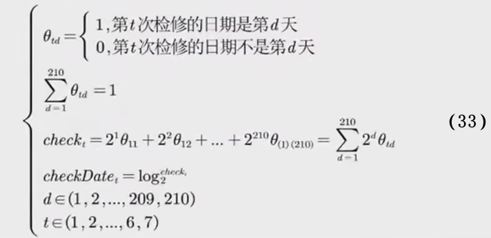
where chechDate t is the specific date of the t-th inspection.
7.1.3 Inspection interval
In order to give the interval of 6 days between two inspection dates more conveniently, the order of 7 inspections is limited first, that is, the checkDate t is sorted first, as follows:
chech D ate i < chech D ate i + 1 , i ∈ ( 1 , 2 , 3...5 , 6 ) (34) chechDate~i~ < chechDate~i+1~ ,i∈(1,2,3...5,6)\tag{34}c h e c h D a t e i <c h e c h D a t e i +1 , i∈( 1 ,2 ,3...5 ,6 )( 34 )
After sorting, a constraint of 6 days between two inspection dates is given, as follows:
c h e c h D a t e i + 6 < c h e c h D a t e i + 1 , i ∈ ( 1 , 2 , 3...5 , 6 ) (35) chechDate~i~ +6< chechDate~i+1~ ,i∈(1,2,3...5,6)\tag{35} c h e c h D a t e i +6<c h e c h D a t e i +1 , i∈( 1 ,2 ,3...5 ,6 )( 35 )
7.1.4 Defining the Total Work Time Limit Matrix
The production time in this question has changed from 7 days to 210 days in 30 weeks, so redefine the total working hours limit matrix:

Among them, T d is the total working hour limit on the d day of the week.
Therefore, the constraints that satisfy the total man-hour limit are as follows:
3 × M A d + 5 × M B d + 5 × M C d ⩽ T b i g d (37) 3 \times MA~d~ +5\times MB~d~ +5\times MC_d\leqslant Tbig_d \tag{37} 3×MA d +5×MB d +5×MCd⩽T be gd( 37 )
7.1.5 Restrictions on total working hours are relaxed after maintenance
After the overhaul of the equipment, the production capacity has been improved. After the first day after the overhaul, the total production time limit is relaxed by 10%, 8%, ..., 2%, and 0%. Therefore, after the specific dates of the 7 inspections are determined, the values in the maximum total man-hour limit matrix can be changed to meet the relaxation after the inspection. Change the formula to look like this:
T b i g ( c h e c h D a t e + o f f s e t ) = T b i g ( c h e c h D a t e + o f f s e t ) × ( 1 + ( 0.1 − 0.02 × o f f s e t ) ) (38) Tbig_{(chechDate+offset)}= Tbig_{(chechDate+offset)} \times (1+(0.1-0.02 \times offset)) \tag{38} T be g(chechDate+offset)=T be g(chechDate+offset)×( 1+( 0.1−0.02×offset))( 38 )
o f f s e t ∈ ( 0 , 1 , . . . 4 , 5 ) offset∈(0,1,...4,5) offset∈( 0 ,1 ,...4 ,5 )
Among them, 1, offset is the date offset, which is offset backward from the date of each maintenance, and the limit relaxation is reduced by 2% for each offset. When the offset reaches 5 times, the limit relaxation is reduced to 0% and the offset is stopped.
7.1.6 No components can be produced on the inspection day
On the day of equipment maintenance, no components can be produced, that is, the output of large components, small components, and robots on the maintenance day is 0, so the constraints are as follows:
M A 1 j = M A 2 j = M A 3 j = M B 1 j = M B 2 j = M C 1 j = M C 2 j = M C 3 j = 0 MA1_j=MA2_j=MA3_j=MB1_j=MB2_j=MC1_j=MC2_j=MC3_j=0 M A 1j=M A 2j=M A 3j=MB 1j=MB2j=MC 1j=MC 2j=MC 3j=0
M A j = M B j = M C j = M W j = 0 (39) MA_j=MB_j=MC_j=MW_j=0 \tag{39} M Aj=MBj=MCj=MWj=0(39)
j ∈ ( c h e c k D a t e t , t ∈ ( 1 , 2 , . . . 6 , 7 ) ) j∈(checkDate_t,t∈(1,2,...6,7)) j∈(checkDatet,t∈( 1 ,2 ,...6 ,7 ))
7.1.7 Ensuring that production can continue
In order to ensure that after the end of 30 weeks and 210 days, the order demand can still be fulfilled on the 31st week Monday, that is, the 211th day, so the production quantity MW of the robot on the 211th day and the remaining quantity SW11- of the robot on the 210th day should not be less than the 211th day. DW.1, the demand quantity of the sky robot, the principle is the same as that of 6.1.5. The constraints are as follows:
M W 211 + S W 211 − 1 ⩾ D W 211 (40) MW_{211}+SW_{211-1}\geqslant DW_{211} \tag{40} MW211+SW211 − 1⩾DW211( 40 )
The question does not give the demand of the robot on the 211th day DW_{211}, here the 30-week Monday data is averaged and rounded to get DW 211 =38.
Other constraints and objective functions have not been changed in the model of problem 2, so they will not be repeated here.
7.2 The solution of the three-model problem
Use MATLAB to write code to obtain the result of question three.
clear
clc
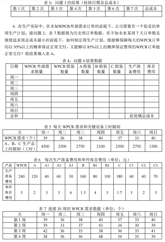
%每天WPCR需求量
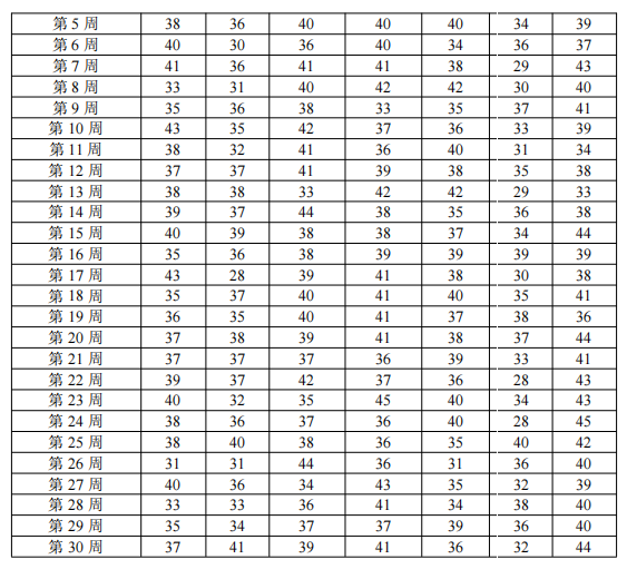
WPCR=[39 36 38 40 37 33 40
39 33 37 43 34 30 39
42 36 35 38 36 35 41
38 36 36 48 34 35 39
38 36 40 40 40 34 39
40 30 36 40 34 36 37
41 36 41 41 38 29 43
33 31 40 42 42 30 40
35 36 38 33 35 37 41
43 35 42 37 36 33 39
38 32 41 36 40 31 34
37 37 41 39 38 35 38
38 38 33 42 42 29 33
39 37 44 38 35 36 38
40 39 38 38 37 34 44
35 36 38 39 39 39 39
43 28 39 41 38 30 38
35 37 40 41 40 35 41
36 35 40 41 37 38 36
37 38 39 41 38 37 44
37 37 37 36 39 33 41
39 37 42 37 36 28 43
40 32 35 45 40 34 43
38 36 37 36 40 28 45
38 40 38 36 35 40 42
31 31 44 36 31 36 40
40 36 34 43 35 32 39
33 33 36 41 34 38 40
35 34 37 37 39 36 40
37 41 39 41 36 32 44];
WPCR=reshape(WPCR',210,1)';
WPCR=[WPCR,WPCR(1:2)];
%一个WPCR队ABC需求比例
A_x=3;
B_x=4;
C_x=5;
D_x=[6;8;2;2;4;8;2;12];
%每天总工时
T=repmat([4500 2500 2750 2100 2500 2750 1500],1,30);
T=[T(end),T,T(1)];
%ABC单位工时消耗
TA=3;
TB=5;
TC=5;
%生产准备费用:A A1 A2 A3 B B1 B2 C C1 C2 C3
W=[240 120 40 60 50 160 80 100 180 60 40 70];
%单件库存费用:A A1 A2 A3 B B1 B2 C C1 C2 C3
C=[5 2 5 3 6 1.5 4 5 1.7 3 2 3];
%模拟退火-粒子群算法
T0=100; %初始化温度值
T_min=1; %设置温度下界
alpha=0.9; %温度的下降率
c1=0.4;c2=0.6; %学习因子
wmax=0.6;wmin=0.4; %惯性权重
num=2; %颗粒总数
X=[];
A=[];
F=[];
for i=1:num
[X(i,:),A(i,:),F(i,1)]=chushihua3(WPCR,A_x,B_x,C_x,T,TA,TB,TC,W,C,D_x);
end
%以最小化为例
[bestf,a]=min(F);
bestx=X(a,:);
bestA=A(a,:);
trace(1)=bestf;
while(T0>T_min)
XX=[];
FF=[];
AA=[];
for i=1:num
[XX(i,:),AA(i,:),FF(i,1)]=chushihua3(WPCR,A_x,B_x,C_x,T,TA,TB,TC,W,C,D_x);
delta=FF(i,1)-F(i,1);
if delta<0
F(i,1)=FF(i,1);
X(i,:)=XX(i,:);
A(i,:)=AA(i,:);
else
P=exp(-delta/T0);
if P>rand
F(i,1)=FF(i,1);
X(i,:)=XX(i,:);
A(i,:)=AA(i,:);
end
end
end
fave=mean(F);
fmin=min(F);
for i=1:num
%权重更新
if F(i)<=fave
w=wmin+(F(i)-fmin)*(wmax-wmin)/(fave-fmin);
else
w=wmax;
end
[~,b]=min(F);
best=X(b,:);%当前最优解
%粒子群算法限制最多找10次位置
m=1;
flag=0;
while flag==1
v=w.*randn(1,28)+c1*rand*(best-X(i,:))+c2*rand*(bestx-X(i,:));%速度
XX(i,:)=round(X(i,:)+v);%更新位置
XX(i,:)=max(XX(i,:),0);%不能小于0
%检验,不满足条件则返回之前的变量
x=reshape(XX(i,:)',7,4)';%重新排列矩阵维度
J=jianyan3(x,AA(i,:),WPCR,A_x,B_x,C_x);
if (length(find((sum(x(2:4,:).*[TA;TB;TC],1)-T)>0))==0 & sum(x(1,:))>=sum(WPCR) & J==0) | m==10
XX(i,:)=X(i,:);
else
m=m+1;
end
end
%计算目标函数
FF(i,1)=fun3(XX(i,:),AA(i,:),WPCR,A_x,B_x,C_x,W,C,D_x);
%更新最优
if FF(i,1)<F(i,1)
F(i,1)=FF(i,1);
X(i,:)=XX(i,:);
A(i,:)=AA(i,:);
end
end
if min(F)<bestf
[bestf,a]=min(F);
bestx=X(a,:);
bestA=A(a,:);
end
trace=[trace;bestf];
T0=T0*alpha;
end
disp('最优解为:')
disp('停检时间')
disp(bestA)
disp('WPCR组装数量、A组装数量、B组装数量、C组装数量,见工作区矩阵zz')
x=reshape(bestx',212,4);
zz=[x(1:210,1),x(2:211,2:4)];
disp('生产准备费用、库存费用见工作区矩阵f1、f2')
[~,f1,f2]=fun3(bestx,bestA,WPCR,A_x,B_x,C_x,W,C,D_x);
disp('总费用')
disp(bestf)
figure
plot(trace)
xlabel('迭代次数')
ylabel('函数值')
title('模拟退火算法')
legend('最优值')
function [X,b,F]=chushihua3(WPCR,A_x,B_x,C_x,T,TA,TB,TC,W,C,D_x)
%初始化变量、计算目标函数值,小件提前两天,大件提前1天
flag1=0;
while flag1==0
%检修
flag3=0;
while flag3==0
    A=zeros(1,length(WPCR));
    a=10+randperm(length(WPCR)-20);
    aa=a(1:7);
    A(aa)=1;
    b=find(A==1);
    c=b(2:end)-b(1:end-1);
    d=find(c<6);
    if length(d)==0
        flag3=1;
    end
end
%检修后提高效率
AA=[];%对应的时间
for i=1:length(b)
    AA=[AA,b(i)+1:b(i)+5];
end
G=repmat([1.1 1.08 1.06 10.4 1.02],1,length(b));
TT=T;
TT(AA)=TT(AA).*G;
X=[];
nn=2;%延迟天数
flag1=1;
KC_WPCR=zeros(1,length(WPCR)+nn);%记录每天WPCR库存
KC=zeros(3,length(WPCR)+nn);%记录每天ABC库存
KC_x=zeros(8,length(WPCR)+nn);%记录每天ABC小件库存
SY_WPCR=zeros(1,length(WPCR)+nn);%记录每天交付WPCR情况
SY=zeros(3,length(WPCR)+nn);%记录每天使用ABC情况
% SY_x=zeros(8,length(WPCR)+nn);%记录每天使用ABC小件情况
SC_WPCR=zeros(1,length(WPCR)+nn);%记录每天组装WPCR情况
SC=zeros(3,length(WPCR)+nn);%记录每天生产ABC情况
SC_x=zeros(8,length(WPCR)+nn);%记录每天生产ABC小件情况
for i=1:length(WPCR)%循环遍历每个WPCR
    if i==1%假设第一天刚好满足WPCR
        sub=[A_x,B_x,C_x].*WPCR(i);%求出每天的WPCR最小ABC需求量
        up=sub;
    else
        sub=max([A_x,B_x,C_x].*WPCR(i)-KC(:,i+nn-1)',0);%除了第一天,每天减去前一天的库存则为当天至少增加的需求量
        up=[];
        up(1)=fix((T(i)-sub([2,3])*[TB;TC])/TA);%BC最低供应时,A最大供应量
        up(2)=fix((T(i)-sub([1,3])*[TA;TC])/TB);%AC最低供应时,B最大供应量
        up(3)=fix((T(i)-sub([1,2])*[TA;TB])/TC);%AC最低供应时,B最大供应量
        up=min(up,fix(T(i)./([A_x,B_x,C_x]*[TA;TB;TC])*2).*[A_x,B_x,C_x]);
    end
    %前面的变量会影响后面的变量范围,可能会出现上up小于sub的情况,毕竟有最大工时限制
    if length(find((up-sub)<0))>0%如果出现则重新生成
        flag1=0;
        continue
    end
    flag2=0;
    while flag2==0
        x=[randi([sub(1),up(1)]),randi([sub(2),up(2)]),randi([sub(3),up(3)])];%在区间内随机生成整数
        if i==1
            flag2=1;
        elseif i>1
            if x*[TA;TB;TC]<=T(i)%需求量必须满足在工时限制内
                flag2=1;
            end
        end
    end
    %每天组装的WPCR
    if i==1
        s=WPCR(i);%可组装最小数量
        u=min(fix(x./[A_x,B_x,C_x]));%可组装最大数量
    else
        s=max(WPCR(i)-KC_WPCR(i+nn-1),0);
        u=min(fix([x+KC(:,i+nn-1)']./[A_x,B_x,C_x]));
    end
    if u<s
        flag1=0;
        continue
    end
    %更新SC、KC、SY矩阵
    %生产
    if length(find(b==i))==1
        SC_WPCR(i+nn)=0;
    else
        SC_WPCR(i+nn)=randi([s,u]);
    end
    if length(find(b==i-1))==1
        SC(:,i+nn-1)=0;
    else
        SC(:,i+nn-1)=SC(:,i+nn-1)+x';
    end
    %放库存
    KC_WPCR(i+nn)=KC_WPCR(i+nn-1)+SC_WPCR(i+nn);
    if KC_WPCR(i+nn)<0
        KC_WPCR(i+nn)=0;
    end
    if i==1
        KC(:,i+nn-1)=SC(:,i+nn-1);
    else
        KC(:,i+nn-1)=KC(:,i+nn-1)+SC(:,i+nn-1);
    end
    KC_x(1:3,i+nn-2)=D_x(1:3).*SC(1,i+nn-1);
    KC_x(4:5,i+nn-2)=D_x(4:5).*SC(2,i+nn-1);
    KC_x(6:8,i+nn-2)=D_x(6:8).*SC(3,i+nn-1);
    %使用
    SY_WPCR(i+nn)=WPCR(i);
    SY(:,i+nn)=[A_x;B_x;C_x].*SY_WPCR(i+nn);
    %更新库存
    KC_WPCR(i+nn)=KC_WPCR(i+nn)-WPCR(i);
    KC(:,i+nn)=KC(:,i+nn-1)-SY(:,i+nn);
end
X=[SC_WPCR(:,nn+1:end);SC(:,nn:end-1)];
X=reshape(X',1,848);
end
X1=[SC_WPCR(:,nn+1:end-2);SC(:,nn+1:end-2)];%生产
X3=[KC_WPCR(:,nn+1:end-2);KC(:,nn+1:end-2)];%库存ABC
X4=[KC_x(:,nn+1:end-2)];%库存ABC小件
X1(find(X1>0))=1;
X2=[repmat(X1(2,:),3,1);repmat(X1(3,:),2,1);repmat(X1(4,:),3,1)];
X2(:,b)=0;
%最优情况,小件无库存但是有生产准备费用
f1=(sum(X1.*[W(1);W(2);W(6);W(9)],1)+sum(X2.*[W(3:5)';W(7:8)';W(10:12)'],1))';
f2=(sum(X3.*C([1,2,6,9])',1)+sum(X4.*C([3,4,5,7,8,10,11,12])',1))';
F=sum(f1)+sum(f2);
function [F,f1,f2]=fun3(X,b,WPCR,A_x,B_x,C_x,W,C,D_x)
%初始化变量、计算目标函数值
X=reshape(X',212,4);
nn=2;
KC_WPCR=zeros(1,length(WPCR)+nn);%记录每天WPCR库存
KC=zeros(3,length(WPCR)+nn);%记录每天ABC库存
KC_x=zeros(8,length(WPCR)+nn);%记录每天ABC小件库存
SY_WPCR=zeros(1,length(WPCR)+nn);%记录每天交付WPCR情况
SY=zeros(3,length(WPCR)+nn);%记录每天使用ABC情况
% SY_x=zeros(8,length(WPCR)+nn);%记录每天使用ABC小件情况
SC_WPCR=zeros(1,length(WPCR)+nn);%记录每天组装WPCR情况
SC=zeros(3,length(WPCR)+nn);%记录每天生产ABC情况
SC_x=zeros(8,length(WPCR)+nn);%记录每天生产ABC小件情况
for i=1:length(WPCR)%循环遍历每个WPCR
    x=X(i,2:4);
    %更新SC、KC、SY矩阵
    %生产
    if length(find(b==i))==1
        SC_WPCR(i+nn)=0;
    else
        SC_WPCR(i+nn)=X(i,1);
    end
    if length(find(b==i-1))==1
        SC(:,i+nn-1)=0;
    else
        SC(:,i+nn-1)=SC(:,i+nn-1)+x';
    end
    %放库存
    KC_WPCR(i+nn)=KC_WPCR(i+nn-1)+SC_WPCR(i+nn);
    if KC_WPCR(i+nn)<0
        KC_WPCR(i+nn)=0;
    end
    if i==1
        KC(:,i+nn-1)=SC(:,i+nn-1);
    else
        KC(:,i+nn-1)=KC(:,i+nn-1)+SC(:,i+nn-1);
    end
    KC_x(1:3,i+nn-2)=D_x(1:3).*SC(1,i+nn-1);
    KC_x(4:5,i+nn-2)=D_x(4:5).*SC(2,i+nn-1);
    KC_x(6:8,i+nn-2)=D_x(6:8).*SC(3,i+nn-1);
    %使用
    SY_WPCR(i+nn)=WPCR(i);
    SY(:,i+nn)=[A_x;B_x;C_x].*SY_WPCR(i+nn);
    %更新库存
    KC_WPCR(i+nn)=KC_WPCR(i+nn)-WPCR(i);
    KC(:,i+nn)=KC(:,i+nn-1)-SY(:,i+nn);
end
X1=[SC_WPCR(:,nn+1:end-2);SC(:,nn+1:end-2)];%生产
X3=[KC_WPCR(:,nn+1:end-2);KC(:,nn+1:end-2)];%库存ABC
X4=[KC_x(:,nn+1:end-2)];%库存ABC小件
X1(find(X1>0))=1;
X2=[repmat(X1(2,:),3,1);repmat(X1(3,:),2,1);repmat(X1(4,:),3,1)];
X2(:,b)=0;
%最优情况,小件无库存但是有生产准备费用
f1=(sum(X1.*[W(1);W(2);W(6);W(9)],1)+sum(X2.*[W(3:5)';W(7:8)';W(10:12)'],1))';
f2=(sum(X3.*C([1,2,6,9])',1)+sum(X4.*C([3,4,5,7,8,10,11,12])',1))';
F=sum(f1)+sum(f2);
function J=jianyan3(X,b,WPCR,A_x,B_x,C_x,D_x)
%检验变量参与运算后是否出现小于0的值,是则不满足条件
X=X';
nn=2;
KC_WPCR=zeros(1,length(WPCR)+nn);%记录每天WPCR库存
KC=zeros(3,length(WPCR)+nn);%记录每天ABC库存
KC_x=zeros(8,length(WPCR)+nn);%记录每天ABC小件库存
SY_WPCR=zeros(1,length(WPCR)+nn);%记录每天交付WPCR情况
SY=zeros(3,length(WPCR)+nn);%记录每天使用ABC情况
SY_x=zeros(8,length(WPCR)+nn);%记录每天使用ABC小件情况
SC_WPCR=zeros(1,length(WPCR)+nn);%记录每天组装WPCR情况
SC=zeros(3,length(WPCR)+nn);%记录每天生产ABC情况
SC_x=zeros(8,length(WPCR)+nn);%记录每天生产ABC小件情况
for i=1:length(WPCR)%循环遍历每个WPCR
    x=X(i,2:4);
    %更新SC、KC、SY矩阵
    %生产
    if length(find(b==i))==1
        SC_WPCR(i+nn)=0;
    else
        SC_WPCR(i+nn)=X(i,1);
    end
    if length(find(b==i-1))==1
        SC(:,i+nn-1)=0;
    else
        SC(:,i+nn-1)=SC(:,i+nn-1)+x';
    end
    %放库存
    KC_WPCR(i+nn)=KC_WPCR(i+nn-1)+SC_WPCR(i+nn);
    if KC_WPCR(i+nn)<0
        KC_WPCR(i+nn)=0;
    end
    if i==1
        KC(:,i+nn-1)=SC(:,i+nn-1);
    else
        KC(:,i+nn-1)=KC(:,i+nn-1)+SC(:,i+nn-1);
    end
    KC_x(1:3,i+nn-2)=D_x(1:3).*SC(1,i+nn-1);
    KC_x(4:5,i+nn-2)=D_x(4:5).*SC(2,i+nn-1);
    KC_x(6:8,i+nn-2)=D_x(6:8).*SC(3,i+nn-1);
    %使用
    SY_WPCR(i+nn)=WPCR(i);
    SY(:,i+nn)=[A_x;B_x;C_x].*SY_WPCR(i+nn);
    %更新库存
    KC_WPCR(i+nn)=KC_WPCR(i+nn)-WPCR(i);
    KC(:,i+nn)=KC(:,i+nn-1)-SY(:,i+nn);
end
if length(find(KC_WPCR<0))>0 | length(find(KC<0))>0 | length(find(KC_x<0))>0
    J=1;
else
    J=0;
end
8. Establishment and solution of the model of the fourth problem
8.1 The establishment of the four model of the problem
8.1.1 Data Analysis
This question needs to predict the use demand of robots in the 31st week. According to the data analysis given by the question, the fluctuation of data has a certain periodicity, and it is period time series data. There is only one dependent variable: the number of robots used. Then, with the number of robots used as the dependent variable, a robot demand prediction model based on univariate time series analysis is established.
Since the data with weeks as the time variable does not give a specific period, consider dividing the data into a training group and an experimental group, use different period lengths to model the training group, screen out the models that pass the Q test, and then use the experimental group's The data determines which model predicts the best. Select the model with the smallest prediction error, use all the data to remodel, and make predictions on future data. Finally, draw the predicted time series diagram to judge whether the predicted trend is reasonable.
8.1.2 Data Preprocessing
Observing data for 30 weeks and 201 days, with no missing data. Define a time variable in weeks, draw a time series graph with time as the horizontal axis and the number of robots as the vertical axis. Analyze the time series graph and find that the data fluctuates up and down within a certain range, without trend or seasonality.
8.1.3 Establishment of prediction model based on univariate time series
The training group data is a sequence with a cycle length of 7, and the optimal time series analysis model is established by using the SPSS expert modeler. The Expert Modeler automatically finds the best fitting model for each dependent sequence. If an independent (predictor) variable is specified, the expert modeler selects for the content in the ARIMA model those models that have a statistically significant relationship to the dependent series. Model variables were transformed using difference or square root or natural log transformations as appropriate. By default, the Expert Modeler considers both Exponential Smoothing and ARIMA models. However, it is also possible to limit the Expert Modeler to search only for ARIMA models or only for exponential smoothing models. You can also specify automatic detection of outliers.
The sPSS Expert Modeler automatically chose the optimal model for us: the simple seasonal model.
8.1.4 Testing of predictive models
Check whether the model is completely recognized: After estimating the time series model, we need to perform a white noise test on the residual. If the residual is white noise, it means that the model we selected can completely identify the law of the time series, that is, the model is acceptable. ; If the residual is not white noise, it means that there is still some information not recognized by the model, then it will be eliminated.
ACF autocorrelation coefficient and PACF partial autocorrelation function can help us determine whether the residual is white noise, that is, whether the time series can be fully recognized by the model.
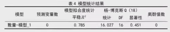
As can be seen from the above table, the p value obtained by the Q-test on the residuals is 0.451, that is, we cannot reject the null hypothesis and think that the residuals are white noise sequences, so the simple seasonal model can well identify the robot in this question. demand data.
Model comparison and selection: Use stationary R 2 or AIC and BIC criteria. R 2 can be used to reflect the quality of linear model fitting, the closer it is to 1, the more accurate the fitting. The more parameters are added, the better the model fitting effect is, but this is at the cost of increasing the complexity of the model (overfitting problem). Therefore, model selection seeks the best balance between model complexity and the ability of the model to interpret the data. Since BIC has a larger penalty coefficient for the complexity of the model, BIC is often more concise than the model selected by AIC. Therefore, the principle of choosing a small R 2 and BIC as the parameters for model selection.
The BIC (Bayesian Information Criterion) expression is as follows:
BIC = ln ( T ) (the number of parameters in the model) - 2 ln (the maximum likelihood function of the model) (41) BIC=ln(T) (the number of parameters in the model) - 2ln (the maximum likelihood of the model) function) \tag{41}BIC=l n ( T ) (number of parameters in the model)−2 l n (maximum likelihood function of the model)( 41 )
Get the predicted values for week 31: 38, 35, 39, 40, 37, 34, 40. Predicted values for the first two days of week 32: 38, 35. Therefore, get the robot demand quantity matrix on the dth day of a week in the future, as follows:
DW predict = [ 38 , 35 , 39 , 40 , 37 , 34 , 40 , 38 , 35 ] (42) DWpredict=[38,35, 39,40,37,34,40,38,35] \tag{42}DWpredict=[ 38 ,35 ,39 ,40 ,37 ,34 ,40 ,38 ,35 ]( 42 )
8.1.5 Guarantee normal delivery every day
In order to ensure that the daily robot orders are delivered with a probability of more than 95%, the constraints on the number of robots assembled are modified as follows:
M W d + S W d − 1 ⩾ D W p r e d i c t d × 0.95 (43) MW_{d}+SW_{d-1}\geqslant DW_{predict_d} \times 0.95 \tag{43} MWd+SWd−1⩾DWpredictd×0.95( 43 )
8.1.6 Guarantee normal delivery throughout the week
In order to ensure that robot orders for the whole week can be delivered with a probability of more than 85%, the following constraints are made:
∑ d = 1 7 M W d ⩾ 0.85 × ∑ d = 1 7 D W p r e d i c t d (44) \sum_{d=1}^7MW_d \geqslant 0.85 \times \sum_{d=1}^7DWpredict_d \tag{44} d=1∑7MWd⩾0.85×d=1∑7DWpredictd( 44 )
It is worth noting that the daily orders have been delivered with a probability of more than 95%, and the robot orders of the whole week must be delivered with a probability of more than 85%, that is, equation (44) has been implied in equation (43). Therefore, it is enough to ensure normal delivery every day, that is, formula (43) can be ignored.
Nine, the official standard answer
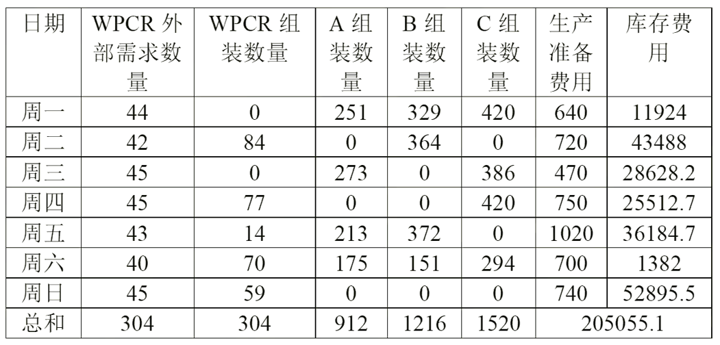
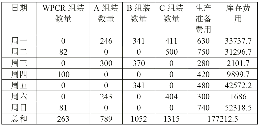
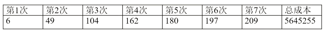
1. The final result of the first question
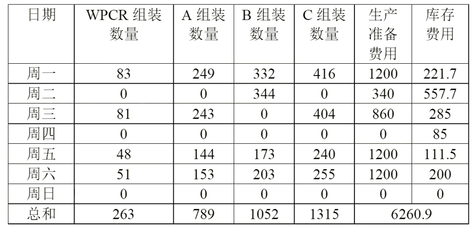
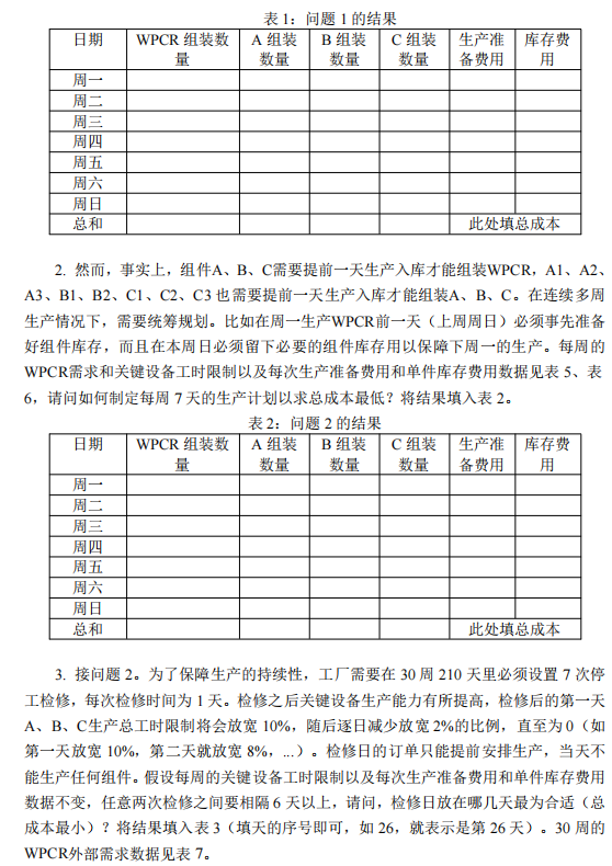
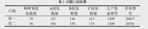
2. The final result of the second question
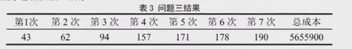
3. The final result of the third question
4. The final result of the fourth question