caffe feature visualization --- python implementation

         Here we mainly test how to visualize the features using caffe's python interface, and extract the convolution kernel and response convolution map in param and blob from a forword. I mainly tested the model and network configuration file under the path of caffe/models/bvlc_reference_caffenet/, the model is bvlc_reference_caffenet.caffemodel, the configuration file is: deploy.prototxt, the model may need to be downloaded by yourself, the download address is http:// dl.caffe.berkeleyvision.org/ , of course, you can also use the model and network configuration file you have trained yourself, the reference code is as follows, pay attention to the corresponding file path:

 caffe_visual.py

# -*- coding:utf-8 -*-

import numpy as np
import matplotlib.pyplot as plt
import them
import caffe
import sys
import pickle
import cv2

caffe_root = '/home/rongsong/Downloads/caffe-caffe-0.15/'   # Your caffe diretory path

deployPrototxt = '/home/rongsong/Downloads/caffe-caffe-0.15/models/bvlc_reference_caffenet/deploy.prototxt'
modelFile = '/home/rongsong/Downloads/caffe-caffe-0.15/models/bvlc_reference_caffenet/bvlc_reference_caffenet.caffemodel'
meanFile = 'python/caffe/imagenet/ilsvrc_2012_mean.npy'
#imageListFile = '/home/chenjie/DataSet/CompCars/data/train_test_split/classification/test_model431_label_start0.txt'
#imageBasePath = '/home/chenjie/DataSet/CompCars/data/cropped_image'
#resultFile = 'PredictResult.txt'

#Network initialization
def use ():
    print 'use ...'
    sys.path.insert(0, caffe_root + 'python')
    caffe.set_mode_gpu()
    caffe.set_device(0)
    net = caffe.Net(deployPrototxt, modelFile,caffe.TEST)
    return net

# Take out the data in params and net.blobs in the network
def getNetDetails(image, net):
    # input preprocessing: 'data' is the name of the input blob == net.inputs[0]
    transformer = caffe.io.Transformer({'data': net.blobs['data'].data.shape})
    transformer.set_transpose('data', (2,0,1))
    transformer.set_mean('data', np.load(caffe_root + meanFile ).mean(1).mean(1)) # mean pixel
    transformer.set_raw_scale('data', 255)  
    # the reference model operates on images in [0,255] range instead of [0,1]
    transformer.set_channel_swap('data', (2,1,0))  
    # the reference model has channels in BGR order instead of RGB
    # set net to batch size of 50
    net.blobs['data'].reshape(1,3,227,227)

    net.blobs['data'].data[...] = transformer.preprocess('data', caffe.io.load_image(image))
    out = net.forward()
    
    #The network extracts the convolution kernel of conv1
    filters = net.params['conv1'][0].data
    with open('FirstLayerFilter.pickle','wb') as f:
       pickle.dump(filters,f)
    vis_square(filters.transpose(0, 2, 3, 1))
    Feature map of #conv1
    feat = net.blobs['conv1'].data[0, :36]
    with open('FirstLayerOutput.pickle','wb') as f:
       pickle.dump(feat,f)
    vis_square (feat, padval = 1)
    pool = net.blobs['pool1'].data[0,:36]
    with open('pool1.pickle','wb') as f:
       pickle.dump(pool,f)
    vis_square (pool, padval = 1)


# The convolution graph sum will be displayed here,
def vis_square (data, padsize = 1, padval = 0):
    data -= data.min()
    data /= data.max()
    
    #Make the composite image square
    n = int(np.ceil(np.sqrt(data.shape[0])))
    padding = ((0, n ** 2 - data.shape[0]), (0, padsize), (0, padsize)) + ((0, 0),) * (data.ndim - 3)
    data = np.pad (data, padding, mode = 'constant', constant_values ​​= (padval, padval))
    #Merge convolutional graphs into one image
    
    data = data.reshape((n, n) + data.shape[1:]).transpose((0, 2, 1, 3) + tuple(range(4, data.ndim + 1)))
    data = data.reshape((n * data.shape[1], n * data.shape[3]) + data.shape[4:])
    print data.shape
    plt.imshow(data)
    plt.show()

if __name__ == "__main__":
   net = use ()
   testimage = '/home/rongsong/Pictures/car0.jpg'     # Your test picture path
   getNetDetails(testimage, net)

The test pictures and results are as follows:

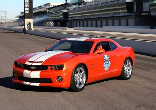
(a) Input test image

                        

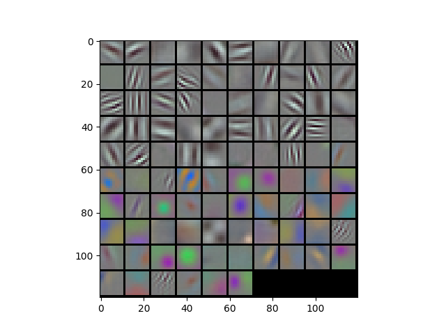
(b) The convolution kernel and convolution graph of the first layer, you can see some obvious edge contours, and the left side is the corresponding convolution kernel

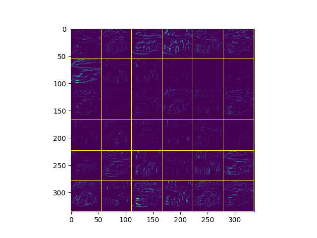
(c) Feature map of the first Pooling layer

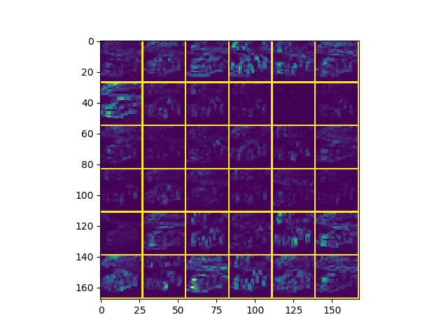
(d) Second-layer convolutional feature map

Reference link: https://www.cnblogs.com/louyihang-loves-baiyan/p/5134671.html