15. Use of Tensorboard

1. Introduction and usage process of TensorBoard

1. Introduction to TensoBoard

TensorBoard and TensorFlow programs run in different processes, and TensorBoard will automatically read the latest TensorFlow log file and present the latest running status of the current TensorFlow program.

2. TensorBoard usage process

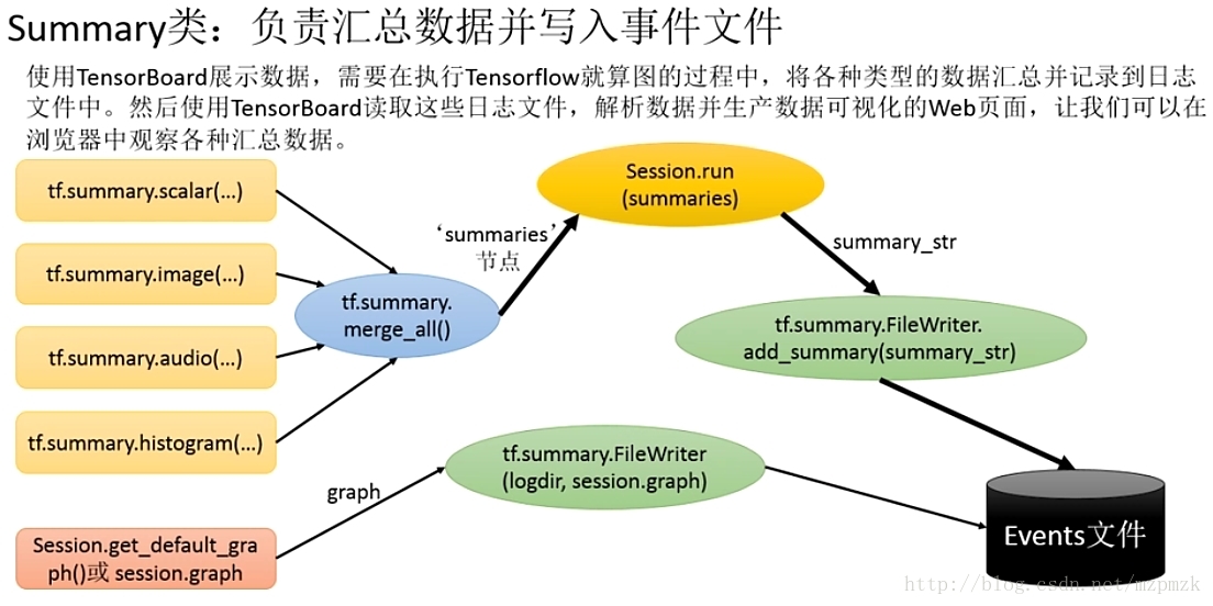
• Add record node: tf.summary.scalar/image/histogram()etc.
• Aggregate record node:merged = tf.summary.merge_all()
• Run the summary node: summary = sess.run(merged), get the summary result
• Log writer instantiation: summary_writer = tf.summary.FileWriter(logdir, graph=sess.graph), pass in graph while instantiating and write the current calculation graph to the log
• summary_writerCall the method of the log writer instance object to add_summary(summary, global_step=i)write all aggregated logs to a file
• summary_writerCall the method of the log writer instance object to close()write to the memory, otherwise it will be written every 120s

---

2. TensorFlow Visual Classification

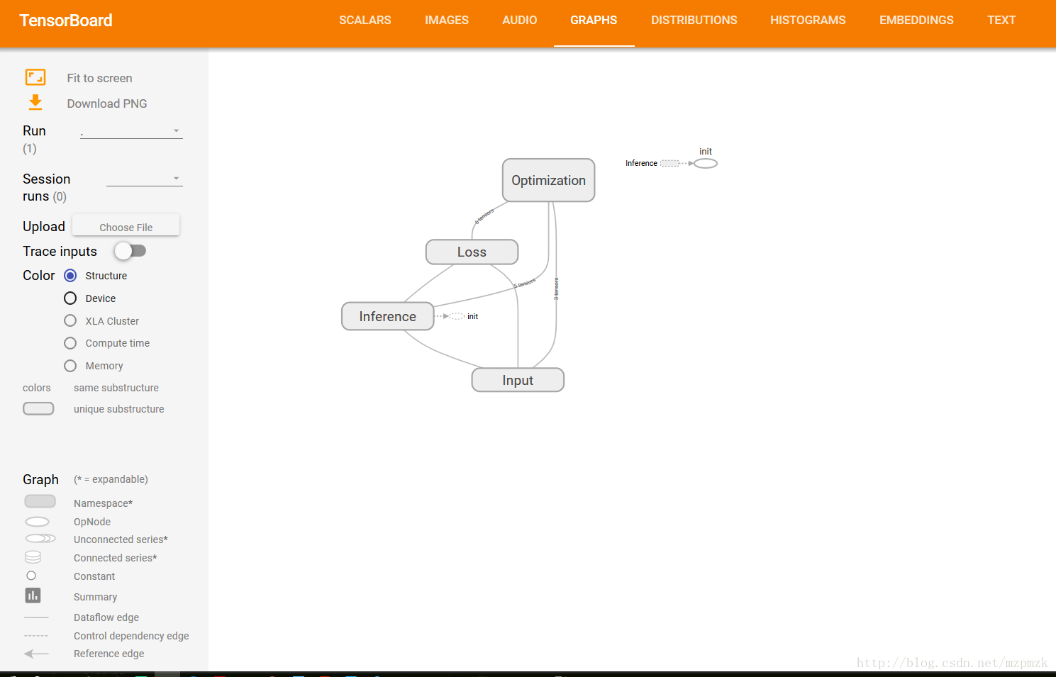
1. Visualization of computational graphs: add_graph()

...create a graph...
# Launch the graph in a session.
sess = tf.Session()
# Create a summary writer, add the 'graph' to the event file.
writer = tf.summary.FileWriter(logdir, sess.graph)
writer.close()  # 关闭时写入内存，否则它每隔120s写入一次

2. Visualization of monitoring indicators: add_summary()

I、SCALAR

tf.summary.scalar(name, tensor, collections=None, family=None)

• Visualize the statistics (mean, std, max/min) of each layer's weight and bias with the number of iterations during the training process: accuracy (val acc), loss value (train/test loss), learning rate (learning rate) ), etc. change curve

• Input parameters:

  • name : The name of this operation node, the vertical axis of the graph drawn in TensorBoard will also use this name
  • tensor : The variable to monitor A real numeric Tensor containing a single value.

• output:

  • A scalar Tensor of type string. Which contains a Summary protobuf.

---

II 、 IMAGE

tf.summary.image(name, tensor, max_outputs=3, collections=None, family=None)

• Visualize 当前轮training/testing images or feature maps used for training

• Input parameters:

  • name : The name of this operation node, the vertical axis of the graph drawn in TensorBoard will also use this name
  • tensor： A r A 4-D uint8 or float32 Tensor of shape [batch_size, height, width, channels] where channels is 1, 3, or 4
  • max_outputs：Max number of batch elements to generate images for

• output:

  • A scalar Tensor of type string. Which contains a Summary protobuf.

---

III、HISTOGRAM

tf.summary.histogram(name, values, collections=None, family=None)

• Visualize the value distribution of a tensor

• Input parameters:

  • name : The name of this operation node, the vertical axis of the graph drawn in TensorBoard will also use this name
  • tensor： A real numeric Tensor. Any shape. Values to use to build the histogram

• output:

  • A scalar Tensor of type string. Which contains a Summary protobuf.

---

IV. Comprehensive summary of a variable

def variable_summaries(var):
    """Attach a lot of summaries to a Tensor (for TensorBoard visualization)."""
    with tf.name_scope('summaries'):
        mean = tf.reduce_mean(var)
        stddev = tf.sqrt(tf.reduce_mean(tf.square(var - mean)))

        # 对变量的均值、标准差、最大(小)值、直方图等进行汇总 
        tf.summary.scalar('mean', mean)
        tf.summary.scalar('stddev', stddev)
        tf.summary.scalar('max', tf.reduce_max(var))
        tf.summary.scalar('min', tf.reduce_min(var))
        tf.summary.histogram('histogram', var)

# 对 activations 中的前 10 张 feature map 进行可视化
tf.summary.image('feature maps', activations, 10)

# 可视化激活前后的直方图
tf.summary。histogram('pre_act', pre_activate)
tf.summary.histogram('act', activations)

---

V 、 MERGE_ALL

tf.summary.merge_all(key=tf.GraphKeys.SUMMARIES)

• Merges all summaries collected in the default graph
• Because there are many log write operations defined in the program, it is very troublesome to call them one by one, so TensorFlow provides this function to organize all log generation operations , eg:merged = tf.summary.merge_all ()
• This operation will not be performed immediately, so you need to explicitly run this operation ( summary = sess.run(merged)) to get aggregated results
• Finally, call the method of the log writer instance object to add_summary(summary, global_step=i)write all the aggregated logs to the file

---

3. Visualization of multiple events: add_event()

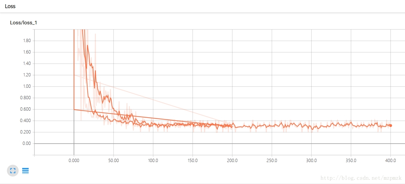
• If the subdirectory of the logdir directory contains data from another run ( multiple events ), then TensorBoard will display all run data (mainly scalar ), which can be used to compare the effects of models with different parameters and adjust the parameters of the model , let it achieve the best effect!
• The line above is the loss curve for 200 iterations, and the bottom line is the curve for 400 iterations . See the procedure at the end.

---

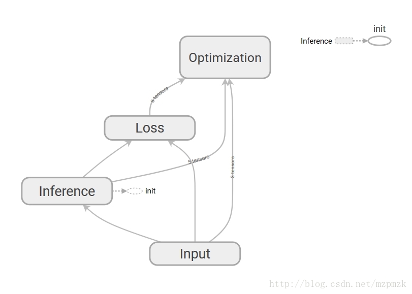
3. Beautify the computational graph through namespaces

• Use namespaces to make visualizations more hierarchical , so that the overall structure of the neural network is not overwhelmed by too many details
• All nodes under the same namespace will be abbreviated as one node , and only nodes in the top -level namespace will be displayed on the TensorBoard visualization
• It can be realized by tf.name_scope()or tf.variable_scope(), see the final procedure for details.

---

Fourth, write all logs to the file: tf.summary.FileWriter()

tf.summary.FileWriter(logdir, graph=None, flush_secs=120, max_queue=10)

• Responsible for writing event logs (graph, scalar/image/histogram, event) to the specified file

• Initialization parameters:

  • logdir : The directory where events are written to
  • graph : If passed in during initialization, it sess,graphis equivalent to calling the add_graph()method for visualization of computational graphs
  • flush_sec：How often, in seconds, to flush the added summaries and events to disk.
  • max_queue：Maximum number of summaries or events pending to be written to disk before one of the ‘add’ calls block.

• Other common methods:

  • add_event(event)：Adds an event to the event file
  • add_graph(graph, global_step=None)：Adds a Graph to the event file，Most users pass a graph in the constructor instead
  • add_summary(summary, global_step=None): Adds a Summary protocol buffer to the event file, be sure to pass in global_step
  • close()：Flushes the event file to disk and close the file
  • flush()：Flushes the event file to disk
  • add_meta_graph(meta_graph_def,global_step=None)
  • add_run_metadata(run_metadata, tag, global_step=None)

---

5. Start TensorBoard to display all log charts

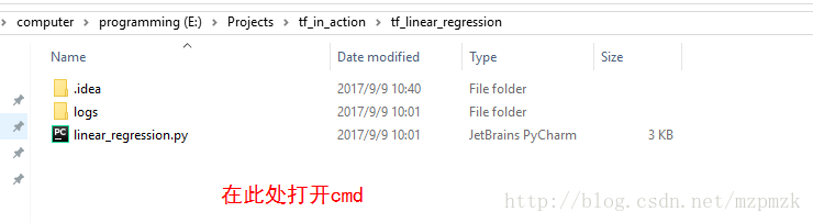
1. Start through cmd under Windows

• Run your program and logsgenerate a eventfile
• In logsthe directory where , hold down the shiftkey, right-click and select open herecmd
• cmdIn , enter the following command to start tensorboard --logdir=logs, note: the directory of logs does not need to be quoted, when there are multiple events in logs, a comparison graph of scalar will be generated, but graph will only display the latest results
• Copy the generated URL ( http://localhost:6006 # 每个人的可能不一样) below to the browser to open it
  
  
  

2. Start via bash under Ubuntu

• Run your program ( ) and generate a file python my_program.pyin the specified directory ( )logsevent
• bashIn , enter the following command to start tensorboard --logdir=logs --port=8888, note: the directory of logs does not need to be quoted, and the port number must be configured in the router in advance
• Copy the generated URL ( http://ubuntu16:8888 # 把ubuntu16 换成服务器的外部ip地址即可) below to your local browser to open it
  

---

6. Use TF to implement univariate linear regression (and visualize it with TensorBoard)

• The comparison diagram of multiple events lossand the network structure diagram ( graph) have been shown above, and will not be repeated here.
• The bottom shows the training process of the network and the final fitting effect diagram

#!/usr/bin/env python3
# -*- coding: utf-8 -*-

import tensorflow as tf
import matplotlib.pyplot as plt
import numpy as np
import os
os.environ['TF_CPP_MIN_LOG_LEVEL'] = '2'


# 准备训练数据，假设其分布大致符合 y = 1.2x + 0.0
n_train_samples = 200
X_train = np.linspace(-5, 5, n_train_samples)
Y_train = 1.2*X_train + np.random.uniform(-1.0, 1.0, n_train_samples)  # 加一点随机扰动


# 准备验证数据，用于验证模型的好坏
n_test_samples = 50
X_test = np.linspace(-5, 5, n_test_samples)
Y_test = 1.2*X_test


# 参数学习算法相关变量设置
learning_rate = 0.01
batch_size = 20
summary_dir = 'logs'

print('~~~~~~~~~~开始设计计算图~~~~~~~~')

# 使用 placeholder 将训练数据/验证数据送入网络进行训练/验证
# shape=None 表示形状由送入的张量的形状来确定
with tf.name_scope('Input'):
    X = tf.placeholder(dtype=tf.float32, shape=None, name='X')
    Y = tf.placeholder(dtype=tf.float32, shape=None, name='Y')


# 决策函数(参数初始化)
with tf.name_scope('Inference'):
    W = tf.Variable(initial_value=tf.truncated_normal(shape=[1]), name='weight')
    b = tf.Variable(initial_value=tf.truncated_normal(shape=[1]), name='bias')
    Y_pred = tf.multiply(X, W) + b


# 损失函数(MSE)
with tf.name_scope('Loss'):
    loss = tf.reduce_mean(tf.square(Y_pred - Y), name='loss')
    tf.summary.scalar('loss', loss)


# 参数学习算法(Mini-batch SGD)
with tf.name_scope('Optimization'):
    optimizer = tf.train.GradientDescentOptimizer(learning_rate).minimize(loss)


# 初始化所有变量
init = tf.global_variables_initializer()


# 汇总记录节点
merge = tf.summary.merge_all()


# 开启会话，进行训练
with tf.Session() as sess:
    sess.run(init)
    summary_writer = tf.summary.FileWriter(logdir=summary_dir, graph=sess.graph)

    for i in range(201):
        j = np.random.randint(0, 10)  # 总共200训练数据，分十份[0, 9]
        X_batch = X_train[batch_size*j: batch_size*(j+1)]
        Y_batch = Y_train[batch_size*j: batch_size*(j+1)]

        _, summary, train_loss, W_pred, b_pred = sess.run([optimizer, merge, loss, W, b], feed_dict={X: X_batch, Y: Y_batch})
        test_loss = sess.run(loss, feed_dict={X: X_test, Y: Y_test})

        # 将所有日志写入文件
        summary_writer.add_summary(summary, global_step=i)
        print('step:{}, losses:{}, test_loss:{}, w_pred:{}, b_pred:{}'.format(i, train_loss, test_loss, W_pred[0], b_pred[0]))

        if i == 200:
            # plot the results
            plt.plot(X_train, Y_train, 'bo', label='Train data')
            plt.plot(X_test, Y_test, 'gx', label='Test data')
            plt.plot(X_train, X_train * W_pred + b_pred, 'r', label='Predicted data')
            plt.legend()
            plt.show()

    summary_writer.close()