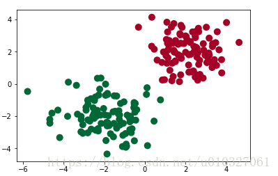
1. Build the dataset:
import torch
from torch.autograd import Variable
import matplotlib.pyplot as plt

# fake data
n_data = torch.ones(100, 2) # basic form of data
x0 = torch.normal(2*n_data, 1)      # 类型0 x data (tensor), shape=(100, 2)
y0 = torch.zeros(100)               # 类型0 y data (tensor), shape=(100, 1)
x1 = torch.normal(-2*n_data, 1)     # 类型1 x data (tensor), shape=(100, 1)
y1 = torch.ones(100)                # 类型1 y data (tensor), shape=(100, 1)

# Note that the data format of x, y data must be as follows (torch.cat is merging data)
x = torch.cat((x0, x1), 0).type(torch.FloatTensor)  # FloatTensor = 32-bit floating
y = torch.cat((y0, y1), ).type(torch.LongTensor)    # LongTensor = 64-bit integer

# torch can only be trained on Variables, so make them Variable
x, y = Variable(x), Variable(y)
#paint
plt.scatter(x.data.numpy()[:, 0], x.data.numpy()[:, 1], c=y.data.numpy(), s=100, lw=0, cmap='RdYlGn')
plt.show()
2. Build a neural network: (the same steps as the previous article regression, modify the number of input and output layers)
import torch
import torch.nn.functional as F # The excitation functions are all here

class Net(torch.nn.Module): # Module that inherits torch
    def __init__(self, n_feature, n_hidden, n_output):
        super(Net, self).__init__() # Inherit __init__ function
        self.hidden = torch.nn.Linear(n_feature, n_hidden) # hidden layer linear output
        self.out = torch.nn.Linear(n_hidden, n_output) # output layer linear output

    def forward(self, x):
        # Forward propagating the input value, the neural network analyzes the output value
        x = F.relu(self.hidden(x)) # excitation function (linear value of hidden layer)
        x = self.out(x) # output value, but this is not the predicted value, the predicted value needs to be calculated separately
        return x

net = Net(n_feature=2, n_hidden=10, n_output=2) # There are several outputs for several categories

print(net) # structure of net
"""
Net (
  (hidden): Linear (2 -> 10)
  (out): Linear (10 -> 2)
)
"""
3. Train the network (modify the cost function)
# optimizer is the training tool
optimizer = torch.optim.SGD(net.parameters(), lr=0.02) # Pass all parameters of net, learning rate,
# When calculating the error, pay attention to the real value! Not! One-hot form, but 1D Tensor, (batch,)
# But the predicted values are 2D tensor (batch, n_classes)
loss_func = torch.nn.CrossEntropyLoss() #Classification is commonly used, and the calculation result is the probability
for t in range(100):
out = net(x) # feed net training data x, output analysis value
loss = loss_func(out, y) # Calculate the error between the two
optimizer.zero_grad() # Clear the residual update parameter value of the previous step
loss.backward() # Error back propagation, calculate parameter update value
optimizer.step() # apply the parameter update value to the parameters of the net
4. Visualization
import matplotlib.pyplot as plt

plt.ion() # draw
plt.show()

for t in range(100):

    ...
    loss.backward()
    optimizer.step()

    # Then go to the top
    if t % 2 == 0:
        plt.cla ()
        # The maximum probability after out of a softmax excitation function is the predicted value
        prediction = torch.max(F.softmax(out), 1)[1]
        pred_y = prediction.data.numpy().squeeze()
        target_y = y.data.numpy()
        plt.scatter(x.data.numpy()[:, 0], x.data.numpy()[:, 1], c=pred_y, s=100, lw=0, cmap='RdYlGn')
        accuracy = sum(pred_y == target_y)/200 # How much of the prediction is the same as the true value
        plt.text(1.5, -4, 'Accuracy=%.2f' % accuracy, fontdict={'size': 20, 'color':  'red'})
        plt.pause (0.1)

plt.ioff() # stop drawing
plt.show()
The above code does not display dynamic images, but displays them one by one.
refer to:
https://blog.csdn.net/qiu931110/article/details/68130199
https://morvanzhou.github.io/tutorials/machine-learning/torch/3-02-classification/
"IndentationError: unexpected indent"解决:https://blog.csdn.net/wuxiaobingandbob/article/details/10379157