Summary: Tensorflow Getting Started Tutorial 1
I bought a few books on tensorflow last year, but when I read it this year, I found that the API used by some sample codes is outdated. It seems like it still makes sense to maintain a tutorial for Tensorflow that is kept up to date. This is the original intention of writing this series.
The fast food tutorial series hopes to lower the threshold as much as possible, talk less, and explain thoroughly.
In order to let everyone see a beautiful scene at the beginning, instead of staying on the long accumulation of basic knowledge, referring to some tutorials on the Internet, we will directly show the example of MNIST handwriting recognition using tensorflow directly from the beginning. Then we will talk about the basics slowly.
Tensorflow Installation Crash Tutorial
Since Python is a cross-platform language, installing tensorflow on each system is relatively easy. We'll talk about GPU acceleration later.
Install tensorflow on Linux platform
We take Ubuntu version 16.04 as an example, first install python3 and pip3. pip is a package management tool for python.
sudo apt install python3
sudo apt install python3-pip
Then you can install tensorflow through pip3:
pip3 install tensorflow --upgradeMacOS install tensorflow
It is recommended to use Homebrew to install python.
brew install python3After installing python3, install tensorflow through pip3.
pip3 install tensorflow --upgradeInstall Tensorflow on Windows platform
It is recommended to install tensorflow through Anaconda on the Windows platform. The download address is: https://www.anaconda.com/download/#windows
Then open Anaconda Prompt and enter:
conda create -n tensorflow pip
activate tensorflow
pip install --ignore-installed --upgrade tensorflow
This will install Tensorflow.
Let's quickly try an example to see if it works:
import tensorflow as tf
a = tf.constant(1)
b = tf.constant(2)

c = a * b

sess = tf.Session()

print(sess.run(c))
The output is 2.
Tensorflow, as the name suggests, is an operation composed of streams of some Tensor tensors.
Operations require a Session to run. If you print(c), you will get
Tensor("mul_1:0", shape=(), dtype=int32)That is to say, this is a multiplication Tensor, which needs to be executed through Session.run().
A Shortcut for Getting Started: Linear Regression
Let's first look at one of the simplest machine learning models, an example of linear regression.
The model for linear regression is simply a matrix multiplication:
tf.multiply(X, w)Then we implement the optimization by calling the function tf.train.GradientDescentOptimizer that Tensorflow computes gradient descent.
Let's take a look at this example code. There are only more than 30 lines, and the logic is still very clear. The example comes from the work of Daniel on github: https://github.com/nlintz/TensorFlow-Tutorials , not my original.
import tensorflow as tf
import numpy as np

trX = np.linspace(-1, 1, 101)
trY = 2 * trX + np.random.randn(*trX.shape) * 0.33 # 创建一些线性值附近的随机值

X = tf.placeholder("float")
Y = tf.placeholder("float")

def model(X, w):
    return tf.multiply(X, w) # X*w线性求值,非常简单

w = tf.Variable(0.0, name="weights")
y_model = model(X, w)

cost = tf.square(Y - y_model) # 用平方误差做为优化目标

train_op = tf.train.GradientDescentOptimizer(0.01).minimize(cost) # 梯度下降优化

# 开始创建Session干活!
with tf.Session() as sess:
    # 首先需要初始化全局变量,这是Tensorflow的要求
    tf.global_variables_initializer().run()

    for i in range(100):
        for (x, y) in zip(trX, trY):
            sess.run(train_op, feed_dict={X: x, Y: y})

    print(sess.run(w))
You will end up with a value close to 2, like 1.9183811 for my run this time
Multiple ways to get handwriting recognition
Linear regression is not addicting, we directly start to perform handwriting recognition in one step.
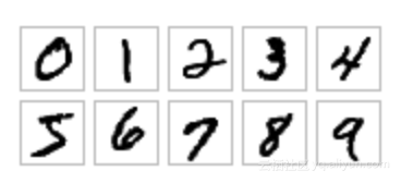
We take the MNIST data of Prof. Yann Lecun, one of the three giants of deep learning, as an example. As you can see in the image above, the data for MNIST is a 28x28 image, and it's labeled what its value should be.
Linear Models: Logistic Regression
First of all, we will use the linear model for classification, regardless of the three-seven-twenty-one.
Counting comments and blank lines, there are about 30 lines in total, and we can solve the difficult problem of handwriting recognition! Please see the code:
import tensorflow as tf
import numpy as np
from tensorflow.examples.tutorials.mnist import input_data

def init_weights(shape):
    return tf.Variable(tf.random_normal(shape, stddev=0.01))

def model(X, w):
    return tf.matmul(X, w) # 模型还是矩阵乘法

mnist = input_data.read_data_sets("MNIST_data/", one_hot=True)
trX, trY, teX, teY = mnist.train.images, mnist.train.labels, mnist.test.images, mnist.test.labels

X = tf.placeholder("float", [None, 784])
Y = tf.placeholder("float", [None, 10])

w = init_weights([784, 10])
py_x = model(X, w)

cost = tf.reduce_mean(tf.nn.softmax_cross_entropy_with_logits(logits=py_x, labels=Y)) # 计算误差
train_op = tf.train.GradientDescentOptimizer(0.05).minimize(cost) # construct optimizer
predict_op = tf.argmax(py_x, 1)

with tf.Session() as sess:
    tf.global_variables_initializer().run()

    for i in range(100):
        for start, end in zip(range(0, len(trX), 128), range(128, len(trX)+1, 128)):
            sess.run(train_op, feed_dict={X: trX[start:end], Y: trY[start:end]})
        print(i, np.mean(np.argmax(teY, axis=1) ==
                         sess.run(predict_op, feed_dict={X: teX})))
After 100 epochs of training, our accuracy is 92.36%.
Brainless shallow neural network
Using the simplest linear model, we replace it with a classical neural network to achieve this function. The graph of the neural network is shown in the figure below.
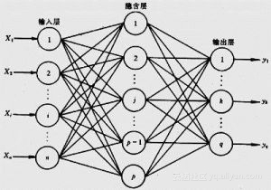
We still ignore the 3721, build a hidden layer, and use the most traditional sigmoid function as the activation function. Its core logic is still matrix multiplication, and there are no tricks in it.
    h = tf.nn.sigmoid(tf.matmul(X, w_h))
    return tf.matmul(h, w_o)
The complete code is as follows, still more than 40 lines, not long:
import tensorflow as tf
import numpy as np
from tensorflow.examples.tutorials.mnist import input_data

# 所有连接随机生成权值
def init_weights(shape):
    return tf.Variable(tf.random_normal(shape, stddev=0.01))

def model(X, w_h, w_o):
    h = tf.nn.sigmoid(tf.matmul(X, w_h))
    return tf.matmul(h, w_o)

mnist = input_data.read_data_sets("MNIST_data/", one_hot=True)
trX, trY, teX, teY = mnist.train.images, mnist.train.labels, mnist.test.images, mnist.test.labels

X = tf.placeholder("float", [None, 784])
Y = tf.placeholder("float", [None, 10])

w_h = init_weights([784, 625])
w_o = init_weights([625, 10])

py_x = model(X, w_h, w_o)

cost = tf.reduce_mean(tf.nn.softmax_cross_entropy_with_logits(logits=py_x, labels=Y)) # 计算误差损失
train_op = tf.train.GradientDescentOptimizer(0.05).minimize(cost) # construct an optimizer
predict_op = tf.argmax(py_x, 1)

with tf.Session() as sess:
    tf.global_variables_initializer().run()

    for i in range(100):
        for start, end in zip(range(0, len(trX), 128), range(128, len(trX)+1, 128)):
            sess.run(train_op, feed_dict={X: trX[start:end], Y: trY[start:end]})
        print(i, np.mean(np.argmax(teY, axis=1) ==
                         sess.run(predict_op, feed_dict={X: teX})))
In the first run, my accuracy was only 69.11% this time, and the second time it was improved to 82.29%. The final result is 95.41%, which is stronger than logistic regression!
Please note that the two lines of code at the core of our model are completely brainless and fully connected to make a hidden layer, and there is no technology in it. It depends entirely on the model ability of the neural network.
Solutions in the Deep Learning Era - ReLU and Dropout
The last time was a bit low-tech, and now is the era of deep learning, and we have made a lot of progress. For example, we know to replace the sigmoid function with the ReLU function. We also knew we were going to do dropout. So we are still a hidden layer and write a more modern model:
    X = tf.nn.dropout(X, p_keep_input)
    h = tf.nn.relu(tf.matmul(X, w_h))

    h = tf.nn.dropout(h, p_keep_hidden)
    h2 = tf.nn.relu(tf.matmul(h, w_h2))

    h2 = tf.nn.dropout(h2, p_keep_hidden)

    return tf.matmul(h2, w_o)
Except for the two tricks of ReLU and dropout, we still have only one hidden layer, and the expressive power is not greatly enhanced. It's not really deep learning.
import tensorflow as tf
import numpy as np
from tensorflow.examples.tutorials.mnist import input_data

def init_weights(shape):
    return tf.Variable(tf.random_normal(shape, stddev=0.01))

def model(X, w_h, w_h2, w_o, p_keep_input, p_keep_hidden):
    X = tf.nn.dropout(X, p_keep_input)
    h = tf.nn.relu(tf.matmul(X, w_h))

    h = tf.nn.dropout(h, p_keep_hidden)
    h2 = tf.nn.relu(tf.matmul(h, w_h2))

    h2 = tf.nn.dropout(h2, p_keep_hidden)

    return tf.matmul(h2, w_o)

mnist = input_data.read_data_sets("MNIST_data/", one_hot=True)
trX, trY, teX, teY = mnist.train.images, mnist.train.labels, mnist.test.images, mnist.test.labels

X = tf.placeholder("float", [None, 784])
Y = tf.placeholder("float", [None, 10])

w_h = init_weights([784, 625])
w_h2 = init_weights([625, 625])
w_o = init_weights([625, 10])

p_keep_input = tf.placeholder("float")
p_keep_hidden = tf.placeholder("float")
py_x = model(X, w_h, w_h2, w_o, p_keep_input, p_keep_hidden)

cost = tf.reduce_mean(tf.nn.softmax_cross_entropy_with_logits(logits=py_x, labels=Y))
train_op = tf.train.RMSPropOptimizer(0.001, 0.9).minimize(cost)
predict_op = tf.argmax(py_x, 1)

with tf.Session() as sess:
    # you need to initialize all variables
    tf.global_variables_initializer().run()

    for i in range(100):
        for start, end in zip(range(0, len(trX), 128), range(128, len(trX)+1, 128)):
            sess.run(train_op, feed_dict={X: trX[start:end], Y: trY[start:end],
                                          p_keep_input: 0.8, p_keep_hidden: 0.5})
        print(i, np.mean(np.argmax(teY, axis=1) ==
                         sess.run(predict_op, feed_dict={X: teX,
                                                         p_keep_input: 1.0,
                                                         p_keep_hidden: 1.0})))
From the results, it can be seen that the accuracy rate of more than 96% has been achieved for the second time. Since then, it has been wandering around 98.4%. Just ReLU and Dropout increased the accuracy from 95% to over 98%.
Convolutional Neural Network Appears
The real deep learning tool CNN, the convolutional neural network comes out. This time the model is indeed a bit more complicated than the previous brainless models. Convolutional layers and pooling layers are involved. This is what we need to talk about in detail later.
import tensorflow as tf
import numpy as np
from tensorflow.examples.tutorials.mnist import input_data

batch_size = 128
test_size = 256

def init_weights(shape):
    return tf.Variable(tf.random_normal(shape, stddev=0.01))

def model(X, w, w2, w3, w4, w_o, p_keep_conv, p_keep_hidden):
    l1a = tf.nn.relu(tf.nn.conv2d(X, w,                       # l1a shape=(?, 28, 28, 32)
                        strides=[1, 1, 1, 1], padding='SAME'))
    l1 = tf.nn.max_pool(l1a, ksize=[1, 2, 2, 1],              # l1 shape=(?, 14, 14, 32)
                        strides=[1, 2, 2, 1], padding='SAME')
    l1 = tf.nn.dropout(l1, p_keep_conv)

    l2a = tf.nn.relu(tf.nn.conv2d(l1, w2,                     # l2a shape=(?, 14, 14, 64)
                        strides=[1, 1, 1, 1], padding='SAME'))
    l2 = tf.nn.max_pool(l2a, ksize=[1, 2, 2, 1],              # l2 shape=(?, 7, 7, 64)
                        strides=[1, 2, 2, 1], padding='SAME')
    l2 = tf.nn.dropout(l2, p_keep_conv)

    l3a = tf.nn.relu(tf.nn.conv2d(l2, w3,                     # l3a shape=(?, 7, 7, 128)
                        strides=[1, 1, 1, 1], padding='SAME'))
    l3 = tf.nn.max_pool(l3a, ksize=[1, 2, 2, 1],              # l3 shape=(?, 4, 4, 128)
                        strides=[1, 2, 2, 1], padding='SAME')
    l3 = tf.reshape(l3, [-1, w4.get_shape().as_list()[0]])    # reshape to (?, 2048)
    l3 = tf.nn.dropout(l3, p_keep_conv)

    l4 = tf.nn.relu(tf.matmul(l3, w4))
    l4 = tf.nn.dropout(l4, p_keep_hidden)

    pyx = tf.matmul(l4, w_o)
    return pyx

mnist = input_data.read_data_sets("MNIST_data/", one_hot=True)
trX, trY, teX, teY = mnist.train.images, mnist.train.labels, mnist.test.images, mnist.test.labels
trX = trX.reshape(-1, 28, 28, 1)  # 28x28x1 input img
teX = teX.reshape(-1, 28, 28, 1)  # 28x28x1 input img

X = tf.placeholder("float", [None, 28, 28, 1])
Y = tf.placeholder("float", [None, 10])

w = init_weights([3, 3, 1, 32])       # 3x3x1 conv, 32 outputs
w2 = init_weights([3, 3, 32, 64])     # 3x3x32 conv, 64 outputs
w3 = init_weights([3, 3, 64, 128])    # 3x3x32 conv, 128 outputs
w4 = init_weights([128 * 4 * 4, 625]) # FC 128 * 4 * 4 inputs, 625 outputs
w_o = init_weights([625, 10])         # FC 625 inputs, 10 outputs (labels)

p_keep_conv = tf.placeholder("float")
p_keep_hidden = tf.placeholder("float")
py_x = model(X, w, w2, w3, w4, w_o, p_keep_conv, p_keep_hidden)

cost = tf.reduce_mean(tf.nn.softmax_cross_entropy_with_logits(logits=py_x, labels=Y))
train_op = tf.train.RMSPropOptimizer(0.001, 0.9).minimize(cost)
predict_op = tf.argmax(py_x, 1)

with tf.Session() as sess:
    # you need to initialize all variables
    tf.global_variables_initializer().run()

    for i in range(100):
        training_batch = zip(range(0, len(trX), batch_size),
                             range(batch_size, len(trX)+1, batch_size))
        for start, end in training_batch:
            sess.run(train_op, feed_dict={X: trX[start:end], Y: trY[start:end],
                                          p_keep_conv: 0.8, p_keep_hidden: 0.5})

        test_indices = np.arange(len(teX)) # Get A Test Batch
        np.random.shuffle(test_indices)
        test_indices = test_indices[0:test_size]

        print(i, np.mean(np.argmax(teY[test_indices], axis=1) ==
                         sess.run(predict_op, feed_dict={X: teX[test_indices],
                                                         p_keep_conv: 1.0,
                                                         p_keep_hidden: 1.0})))
Let's take a look at the running data this time:
0 0.95703125
1 0.9921875
2 0.9921875
3 0.98046875
4 0.97265625
5 0.98828125
6 0.99609375
In the 6th round, it ran a high score of 99.6%, which was greatly improved than the 98.4% of the neural network with one hidden layer of ReLU and Dropout. Because the difficulty is the more difficult it gets.
In the 16th round, I ran out of 100% accuracy:
7 0.99609375
8 0.99609375
9 0.98828125
10 0.98828125
11 0.9921875
12 0.98046875
13 0.99609375
14 0.9921875
15 0.99609375
16 1.0
To sum up, with the help of Tensorflow and machine learning tools, we can solve problems such as handwriting recognition with only a few dozen lines of code, and the accuracy can reach this level.