Face alignment realization plan and realization effect analysis
1. Introduction to Face Alignment
In Face Alignment , traditional methods can achieve good results. However , the effect is not very good in large gestures and extreme expressions . Face alignment can be viewed as searching for predefined points of the face (also called face shape) in a face image, usually starting with a rough estimate of the shape and then iterating to refine the shape estimate. The general framework of its implementation is as follows:
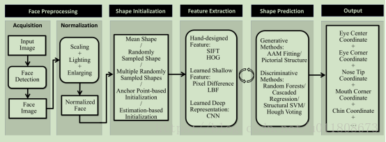
Figure 1.1
The problem of face feature point detection needs to pay attention to two aspects: one is the local feature extraction method at the feature point, and the other is the regression algorithm . The local feature extraction at feature points can also be regarded as a feature representation of the face. The current deep learning -based method can be regarded as first using the neural network to obtain the face feature representation, and then using linear regression to obtain the point coordinates.
2. Deep learning related papers
2.1 Deep Convolutional Network Cascade for Facial Point Detection
The research group of Professor Tang Xiaoou of the Chinese University of Hong Kong proposed a 3 -level convolutional neural network DCNN at CVPR 2013 to realize the method of face alignment. This method can also be unified under the framework of cascaded shape regression model . Unlike CPR , RCPR , SDM , LBF and other methods, DCNN uses a deep model - convolutional neural network to achieve . The first level f1 uses three different regions of the face image (the whole face, eyes and nose regions, nose and lips regions) as input, and trains three convolutional neural networks respectively to predict the location of feature points. The network structure contains 4 convolutional layers, 3 Pooling layers and 2 fully connected layers, and fuse the predictions of the three networks to obtain more stable localization results . The next two stages f2 and f3 extract features near each feature point, and train a convolutional neural network ( 2 convolutional layers, 2 Pooling layers and 1 separately for each feature point )A fully connected layer) to correct the localization results. This method achieved the best localization results at the time on the LFPW dataset.

Figure 2.1
2.2 Coarse-to-Fine Auto-Encoder Networks (CFAN) for Real-Time Face Alignment
A coarse-to-fine autoencoder network ( CFAN ) to describe the complex nonlinear mapping process from face appearance to face shape. The method cascades multiple stacked autoencoder networks , each of which characterizes a partially non-linear mapping from face appearance to face shape. Specifically, inputting a low-resolution face image I , the first-layer autoencoder network f1 can quickly estimate the approximate face shape, denoted as a stack autoencoder network based on global features. The network f1 contains three hidden layers, and the number of hidden layer nodes is 1600 , 900, and 400 respectively . Then improve the resolution of the face image, and extract joint local features according to the initial face shape θ 1 obtained by f1 , and input them to the next layer of autoencoder network f2 to optimize and adjust the positions of all feature points at the same time, denoted as based on Stacked autoencoder network for local features. The method cascades 3 local stacked autoencoder networks {f2, f3, f4} until convergence on the training set. Each local stack self-encoding network contains three hidden layers, and the number of hidden layer nodes is 1296,784,400 respectively . Benefiting from the powerful nonlinear characterization ability of the deep model, the method achieves better performance than DRMF and SDM on XM2VTS , LFPW , HELEN datasets.better results. In addition, CFAN can complete face-to-face alignment in real time ( up to 23 ms / frame on the I7 desktop ), which is faster than DCNN ( 120 ms / frame ).
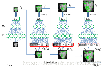
Figure 2.2
3. Current research process
3.1 Implementation scheme Pipline:

Figure 3.1
3.2 Process Analysis
3.2.1 Stage One
a) Resize: Resize the face image to a size of 32*32 , and transform the position of the landmark shape in the same proportion.
b) Landmark selection: Pick out the landmarks of 26 faces ( 21 face edges , 2 remaining eyes , 1 nose , and 2 mouths, expanding the 26 position information is 26*2 = 52 dimensions). Its effect diagram is shown in the figure:

Figure 3.2
c) Landmark shape normalization: The data can be simply processed before training, and the upper left corner of the image can be regarded as coordinates ( -1 , -1 ), and the lower right corner coordinates are regarded as ( 1 , 1 ), so as to recalculate the landmark The location information of the shape .
Note: Some landmarks may not appear in the figure. The location information at this time is represented by ( -1 , -1 ), so in the testing phase, the location information of the small area in the upper left corner should be discarded.
Discard rules: 
d) Selection of activation function, in order to better fit our position information, we use the tanh function as the activation function. Since our position information is [-1,1] , it is easier to converge with tanh . [ Of course, the sigmoid activation function can also be used here , then when the corresponding landmark shape is normalized, the upper left corner of the image should be regarded as (0 , 0) , and the lower right corner should be regarded as (1 , 1)) Discarding rules: or directly Use the RELU function , so you don't have to normalize the location information of the landmark shape ]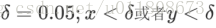
e) The tanh function image is shown in the following figure:
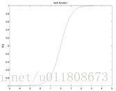
Figure 3.3
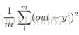
f) Loss adopts EuclideanLoss, the formula is as follows.
Tip : If you want to improve the accuracy of the edge, you can set a larger error ratio for the edge points , eg 
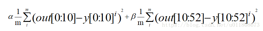
Among them, [0:10] represents the 5 landmarks of the eyes, nose and mouth , and [10:52] represents the 21 landmarks on the edge of the face
3.2.2 Stage two
a) Resize: Resize the face image to a size of 96*96 , and transform the position of the landmark shape in the same proportion.
b) Training data preparation, the training data is divided into 4 parts, namely the left eye, the right eye, the nose, and the mouth. There are several methods for preparing the training data in the second stage.
l Based on the five output results of the first stage as the center, the region is clipped, and the clipping width and height are [48 , 36]. After clipping, the landmark shape position information needs to be transformed by the c-th step of stage one .
l Based on the marked data, region clipping and landmark shape location information transformation are performed according to the marked information. The clipping center can be transformed in a small range to simulate the real stage one result.
c) Landmark normalization, activation function, and loss function are consistent with stage one .
d) During training, the patch image channels of the 4 parts are first fused. The result of the fused image is: [48, 36, 3*4], if the image channel fusion is not performed here, 4 CNN networks are used for regression respectively . , in theory, there will be a more accurate regression effect, but it is more troublesome to train, so the fusion method is adopted, so that only one CNN network is trained for regression.
3.3 Test results
Combine the detection results of Stage One and Stage Two .
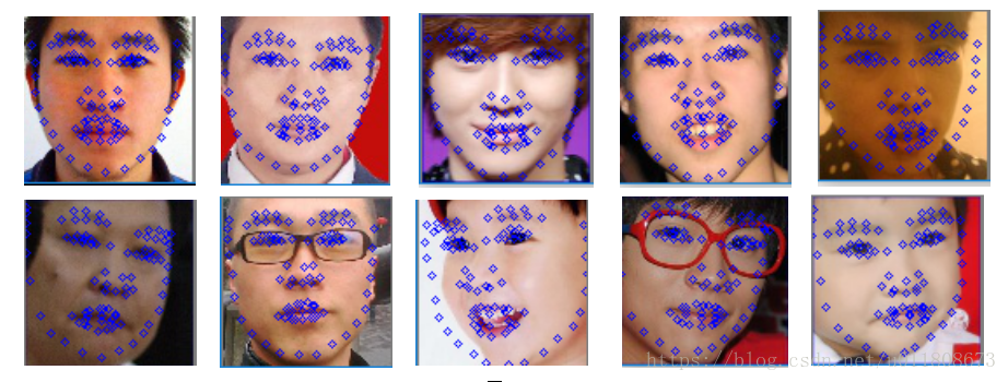
Figure 3.4
It can be seen from the figure that the effect of the edge detection of the profile face is not as accurate as that of other landmark positions , mainly because , in order to speed up the regression , the edge information only undergoes a regression based on the global image features.
4. Training
4.1. Training configuration
base_lr: 0.00001
lr_policy: "inv"
gamma: 0.0001
power: 0.75
regularization_type: "L2"
weight_decay: 0.0005
momentum: 0.9
max_iter: 20000
4.2 Model diagram
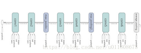
Figure 4.1
5. Error analysis
5.1 Error loss calculation
The test error evaluation standard formula is as follows:
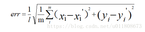
Where l is the length of the face frame , m is the number of landmarks .
5.2 Convergence of Loss function
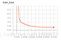
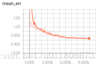
Figure 5.1
Here train_loss adds a weight parameter of 5 times , so the final value is larger than the value of test_loss .