SciML solves simple pendulum problem

The pendulum problem can be expressed as

$$\ddot{\theta }+\frac{g}{L}\mathrm{without}\theta =0$$

Among them, $g$ is the acceleration of gravity;$L$ is the pendulum length;$\theta$ is the swing angle, there is no analytical solution to this equation.

When the angle is relatively small, $\sin \left(\theta \right)\approx \theta$ , then the pendulum problem can be reduced to a linear form

$$\ddot{\theta }+\frac{g}{L}\theta =0$$

When the angle is large, it can be solved numerically. First, split it into a system of first-order differential equations

$$\begin{array}{rl}& \dot{\theta }=\omega \\ & \dot{\omega }=-\frac{g}{L}\mathrm{without}\end{array}$$

using OrdinaryDiffEq, Plots
plotlyjs()

const g = 9.81  #g是常量
L = 1.0

u₀ = [0,π/2]
tspan = (0.0,6.0)

#定义问题
function simplependulum(du,u,t)
    θ = u[1]
    ω = u[2]        #\omega + tab = ω
    du[1] = ω
    du[2] = -(g/L)*sin(θ)
end

prob = ODEProblem(simplependulum, u₀, tspan)
sol = solve(prob,Tsit5())

# plotlyjs绘图面板中有个相机的图标，点击可保存图片
plot!(sol, title ="钟摆问题", xaxis = "时间", label = ["θ" "ω"])

as the picture shows

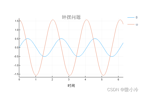
Among them Tsit5is a solver for a system of first-order nonlinear differential equations, which has been used before for solving decay curves, but is not described. Tsit5It is the preferred solver recommended by SciML, the 5th-order Tsitouras method, and an improved Runge-Kutta method.

In physics, in addition to establishing the relationship between physical quantities over time, it is sometimes necessary to establish the relationship between physical quantities, especially the relationship between velocity and coordinates, which constitute all possible states of the system, commonly known as phase space.

In three-dimensional space, velocity and momentum have three directions respectively, so the phase space in three-dimensional space generally has six dimensions. But for the wobble problem, velocity and position can be reduced to one dimension, so the phase space has two dimensions.

Since our drawing space also has two dimensions, only lines can be drawn, that is, only some lines can be drawn from the phase space.

p = plot(sol,vars = (1,2), xlims = (-15,15), title = "相空间", xaxis = "速度", yaxis = "位置", leg=false)
# 用于绘图的函数
function phase_plot(func, u0, p)
    prob = ODEProblem(func,u0,(0.0,2pi))
    sol = solve(prob,Vern9()) # Vern9精度更高
    plot!(p,sol,vars = (1,2))
end
for i in -4pi:pi/2:4π
    for j in -4pi:pi/2:4π
        phase_plot(simplependulum, [j,i], p)
    end
end
plot(p,xlims = (-15,15))

The result is as follows