Preface
This article is the accompanying notes for the open class "Introduction to MIT Algorithms" at station B. Friends who have questions about the content and format of the notes are welcome to communicate in private messages or in the comment area~
The quick sort algorithm is also one of the applications of the divide and conquer algorithm , and it is sorted in place (rearranging elements in the original data area), and the quick sort is also very practical .
1. Description of Quick Sort
- Divide and conquer strategy in fast queue
①Divide
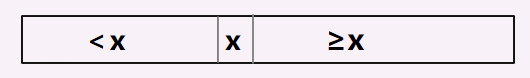
Select a key element, and divide the array into two sub-array parts according to the size of the key element, the left sub-array is smaller than the key element; the element in the right sub-array ≥ the key element.
②Conquer
Recursively handle the sorting problem of two sub-arrays
③Combine
In the quick sorting problem, combining this step is not very important, because when the division is completed and the sorting problem of the two sub-arrays is processed recursively, the entire array is already in order.
The most important step in fast sorting is the partition step-find a segmentation element and divide the entire array into two sub-arrays.
From this perspective, you can understand the fast sorting problem as continuously dividing the array recursively.
- Pseudo-code representation of quick sort
(1)partition()
int Partition(int A[],int p,int q){


  x ← A[p]
  i ← p
  for j ← P+1 to q
    do if A[j]≤x
      then i ← i+1
      exch(A[i],A[j])
  exch(A[p],A[i])
  return i
The main idea of the above code:
- Each time the first element of the array is selected as the split element, the pointer i and the previous save all elements that are less than or equal to the split element; the pointers i to j store all the elements greater than or equal to the split element; the elements after the pointer j Is an element that has not yet been compared
- Each time an element is reviewed, if the element is greater than the segmented element, the pointer j can continue to move backward; if the current element is smaller than the segmented element, the current element and the element pointed to by i+1 are exchanged (according to the first point, the pointer i The element pointed to by +1 must be the first element currently compared that is greater than the segmented element), and then move the pointers i and j back by one bit.
- After the final loop is completed, the segmented element is exchanged with the element pointed to by the pointer i, and the index i is returned as the index after the round of segmentation.
The pseudo-code idea given in the book "Introduction to Algorithms" is the same, except that the last element of the array is selected as the segmentation element.

The partition examples I came across in the algorithm class are roughly the same-choose the segmentation element, and then maintain the pointer to compare with the segmentation element, and exchange the elements that do not match the size relationship. But at that time it was scanning at the same time with two pointers
int partition(int a[],int lo, int hi){


    int i = lo,j = hi+1;
    int v = a[lo];//切分元素
    while(true){


      while(less(a[++i],v) if(i == hi) break;
      while(less(v,a[--j])) if( j == lo) break;
      if( i >= j) break;//当指针i和j相遇时主循环就会退出
      exch(a,i,j);
      }
    exch(a,lo,j);//将v = a[j]放入正确的位置
    return j;
    }
- In the loop, when a[i] is less than v, we increase i, when a[j] is greater than v, we decrease j, and then exchange a[i] and a[j] to ensure that none of the elements on the left of i Greater than v, the elements on the right side of j are not less than v.
- When the pointers meet, swap a[lo] and a[j], and the split ends-so that the split value stays in a[j].
The partition implementation code excerpted in the book of Algorithms, in order to pursue symmetry, has some special subscript initialization, so there is no need to go into it.
Regardless of the implementation, the time complexity of the segmentation process is probably maintained at θ(n), because the entire process is equivalent to traversing all the elements in the array.
(2)quicksort()

(3) Improve tips
①Adjust the code "if(p <q)":
When the code is if(p<q), it means that there is no workload when the processed array has 0 or 1 elements.
This can be improved to find a suitable algorithm to improve the efficiency of sorting when the number of elements is small.
[This point is also implemented in the improvement of the merge algorithm " Implementation and Analysis of the Merge Sort Algorithm" ]
②According to the pseudo-code of fast sorting, we can know that the algorithm is tail-recursive, so some tail-recursive optimization procedures can be used.
For some concepts of tail recursion, please refer to [Allen Chou] this blogger’s article "Explaining what is tail recursion (easy to understand, example explanation)"
- Example of fast queue

Description: The above process is based on the implementation of partition, that is, the last element of the array is selected as the result of the split element.
2. Analysis of the complexity of fast sorting
First, I will give a conclusion. This section will carry out a lot of "interesting" derivation processes for complex
The running time of quick sort is related to whether the partition is symmetric, and whether the partition is symmetric to a large extent depends on which partition element is selected.
If the division is symmetric, then the fast sort has the same complexity as the merge sort in the progressive sense;
if the division is asymmetric, then the fast sort has the same complexity as the insertion sort in the progressive sense.
1. Worst case classification
The worst-case division behavior of fast sorting occurs when the two regions generated by the division process contain n-1 elements and 1 0 element respectively (from the perspective of the entire array, that is, when the entire array is in order or reverse order) .
Assuming that each division uses an asymmetric division, and the time cost of division is θ(n), and the cost T(0) of recursive calls to a zero-element array is set to θ(1), then:

then the algorithm runs The recursive expression of time is shown in the figure below:

Intuitively, if the cost of each layer of recursion is added, an arithmetic progression should be obtained, so that it can be deduced that the cost is square.
It can be seen that the average performance of fast sorting is consistent with the average performance of insertion sort in the worst case. Even when the elements are all ordered, insertion sort only requires linear time complexity O(n).
The recursion tree looks like this:

The ps graph is a bit high and ambiguous, please forgive
the recursive tree obtained in the above figure (the structure is very unbalanced), the height of the tree is n (because each layer is reduced by one), the sum of the complexity of all root nodes is added It is the square level, the complexity of all leaf nodes (a total of n) is θ(1), and the sum is linear level.
So the total sum is θ(n 2 )+θ(n) = θ(n 2 ).
2. Best case analysis
(1) Complexity recurrence formula
In the most balanced division obtained in the division step, the size of the two sub-problems obtained cannot be larger than n/2. In this case, the quick sort operation speed is much faster.
To derive the complexity recursive formula at this time, there are:

(2) Balanced division
Even when we know that the worst-case scenario of fast sorting is the complexity of the square level, we still highly approve the efficiency of fast sorting, because from the average situation, the efficiency of fast sorting is also linear logarithmic level.
The average case of fast sorting is close to the running time of the best case, not the running time of the worst case; to understand this, it is necessary to understand how the balance of division is reflected in the recursive expression that characterizes the running time.
Assuming that the division process always produces a 9:1 division
, the recursive formula of complexity is written as:
T(n) = T(n/10)+T(9n/10)+θ(n) ≤ T(n/10) )+T(9n/10)+cn
To build a recursive tree for the above recursive formula, the tree height and the calculation cost of each layer are shown in the figure below.

According to the structure of the tree, the overall complexity can be analyzed, T(n)≤c·n·log 10/9 n +θ(n), the complexity of this formula in the asymptotic sense is O(nlogn)
From the perspective of mathematical calculations, no matter what the base of logarithmic operations is, the base can be converted to 2 through the nature of logarithmic operations, and then the excess terms are added to the entire logarithmic term as coefficients.
3. Average situation analysis
In order to have a clearer understanding of the average situation of quick sort, it is necessary to make an assumption about the frequency of occurrence of various inputs.
But when applying quick sort to a random input array, it is impossible to assume that each layer has the same division and distribution. We can only expect that some divisions are more balanced, and some divisions are unbalanced.
Suppose that good partitions and bad partitions appear alternately at each level of the tree:
we can get two sets of recursive and recursive trees
L(n) = 2U(n/2) + θ(n)-------Lucky
U(n) = L(n-1) + θ(n) -------Unlucky

【Use Substitution Method and Main Theorem]

How to ensure that we can always have asymptotically optimal complexity?
- Shuffle the elements in the array randomly
- Randomly choose to divide the pivot
We usually consider the latter because it is more convenient and intuitive to analyze.
3. Randomized version of fast sorting
"In many cases, we can add randomization components to an algorithm so that it can obtain better average performance for all inputs."
-The randomized version of fast sorting is ideal for large enough inputs.
[Random sampling]
Instead of always using A[r] as the pivot, an element is randomly selected from the sub-array A[p...r], that is, A[r] and A[p...r] are randomly selected Exchange one element out, and then perform quick sorting according to the previous logic.
In the above randomization operation, we randomly sample from the range of p,...r, so as to ensure that among the r-p+1 elements of the sub-array, the pivot element x = A[r], etc. Take any one of them.
Because the pivot elements are randomly selected, we expect that on average, the division of the input array can be more symmetrical.
1. The advantages of randomized fast sorting:
①The running time does not depend on the order of the input sequence.
②There is no need to make any assumptions about the distribution of the input sequence.
③There will be no specific input that leads to the worst case. The worst case is only determined by the random number generator.
2. Randomize the pseudo-code of fast sorting
