Geometry in opendrive

The direction of the road can be varied, it can be a straight line on an open ground, a long and thin curve on a highway, or a narrow turn in a mountainous area. In order to correctly model all these road lines from a mathematical point of view, OpenDRIVE provides a variety of geometric shape elements. Figure 19 shows five possible ways to define the geometry of the road reference line:

straight line
Spiral or cyclotron curve (curvature changes in a linear manner)
An arc of constant curvature
Cubic polynomial curve
Parametric cubic polynomial curve

1 Road reference line

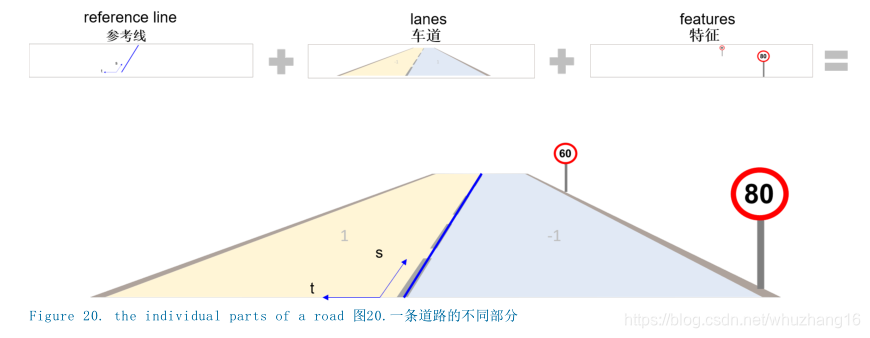
The road reference line is the basic element of each road in OpenDRIVE. All geometric elements that describe the shape of the road and other attributes are defined in accordance with the reference line. These attributes include lanes and signs.

By definition, the reference line stretches in the s direction, while the object is laterally offset from the reference line and stretches in the t direction.

Figure 20 shows the different parts of a road in OpenDRIVE.

Road reference line
Separate lane on a road
Road features (such as signs) placed along the road

In OpenDRIVE, the geometry of the reference line is represented by the <geometry> element in the <planView> element.

The <planView> element is an element that must be used in every <road> element.

The following rules apply to road reference lines:

Every road must have a reference line.
There can only be one reference line for each road.
The reference line is usually at the center of the road, but it may also have a lateral offset.
The geometric elements should be arranged in ascending order (ie, increasing s positions) along the reference line.
A <geometry> element should only contain an element that additionally describes the geometric shape of the road.
If two roads are not connected by an intersection, the reference line of the new road should always start from the <contactPoint> of its predecessor or successor road. The reference line may be pointed in the opposite direction.
The reference line must not have leaps.
The reference line should not have kinks.

2 straight

In OpenDRIVE, straight lines are represented by the <line> element in the <geometry> element.

XML example

<planView>
<geometry
s="0.0000000000000000e+00"
x="-4.7170752711170401e+01"
y="7.2847983820912710e-01"
hdg="6.5477882613167993e-01"
length="5.7280000000000000e+01">
<line/>
</geometry>
</planView>

3 Spiral

As shown in Figure 23, the spiral is a convolute curve describing the curvature of the reference line. Spiral lines can be used to describe the continuous transition of curvature from <line> to <arc>.

The spiral is characterized by the curvature of the starting position (@curvStart) and the curvature of the ending position (@curvEnd). The arc length along the spiral (see the <geometry> element @length), the curvature is linear from beginning to end.

You can also arrange the elements of <line>, <spiral> and <arc> in order to describe the complex curvature.

In OpenDRIVE, the spiral is represented by the <spiral> element in the <geometry> element.

XML example

<geometry s="100.0" x="38.00" y="-1.81" hdg="0.33" length="30.00">
    <spiral curvStart="0.0" curvEnd="0.013"/>
</geometry>

The following rules apply to spirals:

@curvStart and @curvEnd should not be the same.

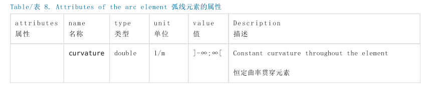
4 arc

As shown in Figure 24, the arc describes the road reference line with constant curvature.

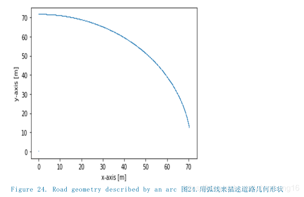
In OpenDRIVE, the arc is represented by the <arc> element in the <geometry> element.

XML example

<planView>
<geometry
s="3.6612031746270386e+00"
x="-4.6416930098385274e+00"
y="4.3409250448366459e+00"
hdg="5.2962250374496271e+00"
length="9.1954178989066371e+00">
<arc curvature="-1.2698412698412698e-01"/>
</geometry>
</planView>

The following rules apply to arcs:

The curvature should not be zero.

5 Generate arbitrary lane lines from geometric shape elements

As shown in Figure 25, by combining all available geometric shape elements in OpenDRIVE, many types of road lines can be created.

In order to avoid fractures in the curvature, it is recommended to use spirals to combine straight lines with arcs and other elements with different curvatures.

6 cubic polynomial (deprecated)

The third-degree polynomial can be used to generate complex road directions derived from measurement data. The measurement pair defines the polynomial limit of the line segment in the specified order of the measured coordinates along the reference line in the x/y coordinate system.

The local cubic polynomial describes the reference line of the road. By specifying the continuity conditions at the limit of the line segment, such as line segment continuity, tangent and/or curvature continuity, etc., multiple cubic polynomial line segments can be merged and a global cubic spline interpolation curve can be generated for the entire road direction. Another advantage is that the path along the polynomial is more efficient than along the cyclotron curve.

6.1 Background information on cubic polynomials

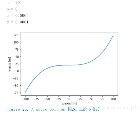
The following equation describes the interpolation of the cubic polynomial in the x/y coordinate system:
y(x) = a + b*x + c*x2 + d*x³

The polynomial parameters a, b, c, and d in the formula are used to define the direction of the road. With the aid of the parameter ad, the y coordinate of each point in the coordinate system can be calculated from the x coordinate.

Figure 26 shows the cubic polynomial in the x/y coordinate system using the following values:

6.2 Use cubic polynomials to create roads

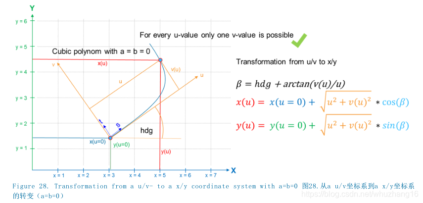
As shown in Figure 27, the cubic polynomial described in the x/y coordinate system is not suitable for describing curve segments with arbitrary directions. In order to process a curve segment with two or more y coordinates on a given x coordinate, the cubic polynomial segment may be defined according to the relationship with the local u/v coordinate system. The use of local u/v coordinate system improves the flexibility of curve definition. The following equation is used:
v(u) = a + b*u + c*u2 + d*u³

The direction of the local u/v coordinate system should be selected in the following way: the function v(u) on the increasing u coordinate is used to express the curve.

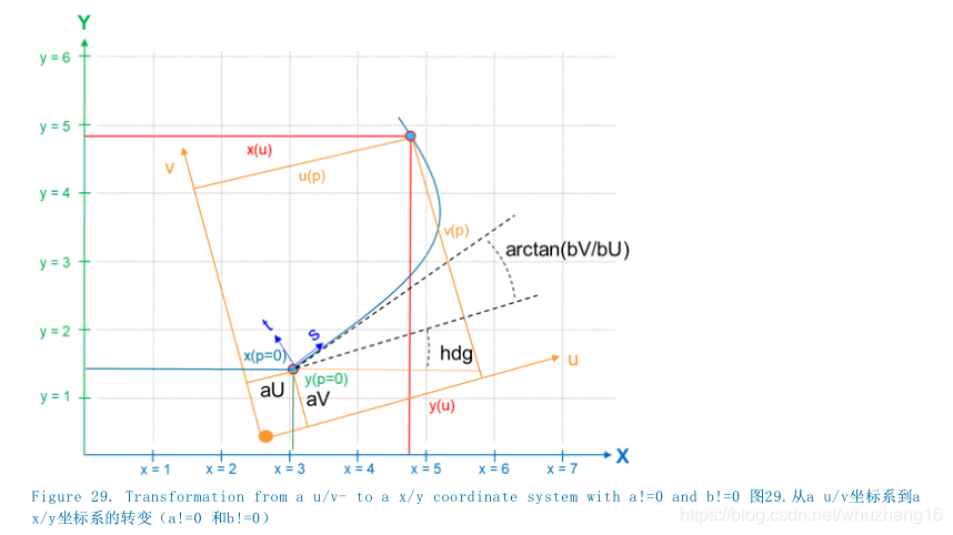
Generally speaking, u/v coordinate system and s/t coordinate system are on the starting position (@x,@y) and starting direction @hdg of the line segment (the two points are detailed in the <geometry> element) Is consistent. The result of this choice is the polynomial parameter a=b=0 (see Figure 28). As an additional option, the local u/v coordinate system can be rotated relative to the starting point (@x,@y) by specifying a polynomial parameter @b that is not equal to 0. Here, the arc tangent arctan(@b) defines the heading/yaw angle of the polynomial relative to the local u/v coordinate system. A polynomial parameter @a that is not equal to 0 (see Figure 29) can be set to obtain
the additional displacement of the origin of the u/v coordinate system along the v coordinate axis when (@x,@y) should be positioned at u=0 . The parameter u may change with the projection from 0 to the end of the curve on the u coordinate axis. For a given parameter u, the local coordinate v(u) defines the point on the curve in the local u/v coordinate system.
v(u) = a + b*u + c*u2 + d*u³

Taking into account the displacement and rotation parameters @a, @b, (@x,@y) and @hdg specified in the <geometry> element, the final x/y curve position on the given u coordinate is shown in Figure 29.

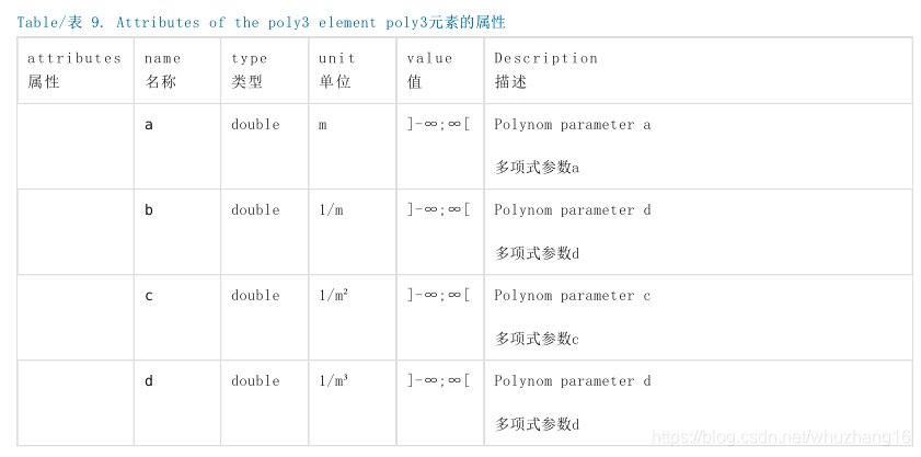
In OpenDRIVE, the cubic polynomial is represented by the <poly3> element in the <geometry> element.

XML example

<geometry
s="0.0000000000000000e+00"
x="-6.8858131487889267e+01"
y="4.1522491349480972e-01"
hdg="6.5004409066736524e-01"
length="2.5615689718113455e+01">
<poly3
a="0.0000000000000000e+00"
b="0.0000000000000000e+00"
c="1.4658732624442020e-02"
d="-5.7746497381565959e-04"/>
</geometry>
<geometry
s="2.5615689718113455e+01"
x="-4.8650519031141869e+01"
y="1.5778546712802767e+01"
hdg="2.9381264033570398e-01"
length="3.1394863696852912e+01">
<poly3
a="0.0000000000000000e+00"
b="0.0000000000000000e+00"
c="-1.9578575382799307e-02"
d="2.3347864348004167e-04"/>
</geometry>

The following rules apply to cubic polynomials:

The third-degree polynomial may be used to describe the course of the road when the measurement data is available.
If the local u/v coordinate system is consistent with the starting point of the s/t coordinate system, then the polynomial parameter coefficient is a=b=0.
The starting point (@x,@y) of the <geometry> element is positioned on the v axis of the local u/v coordinate system.
The polynomial parameters a and b should be 0 to ensure the smoothness of the reference line.

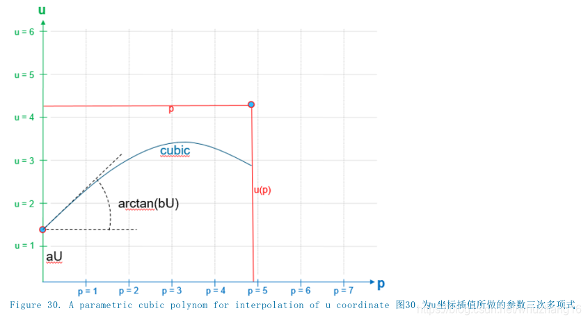
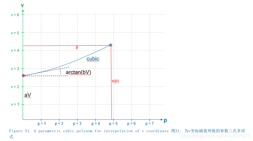
7 Parametric cubic curve

The parametric cubic curve is used to describe the complex curve generated from the measurement data. The parametric cubic curve is more flexible than the cubic polynomial, and it can describe more kinds of road lines. Compared with the cubic polynomial defined in the x/y coordinate system or regarded as the local u/v coordinate system, the interpolation of the x coordinate and the y coordinate is performed by their own splines relative to the common interpolation parameter p.

7.1 Use parametric cubic curve to generate road

You can use parametric cubic curves to generate road lines just by using the x-axis and y-axis. In order to maintain the continuity of the third-degree polynomial, the u-axis and v-axis can be used to calculate them into the third-degree polynomial at the same time.

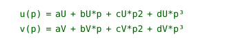
Unless otherwise specified, the interpolation parameter p is in the range of [0;1]. In addition, it can also be assigned within the range of [0; @length of <geometry> ]. Similar to the cubic polynomial, the local coordinate system with variables u and v can be placed and rotated arbitrarily.

To simplify the description, the local coordinate system can be consistent with the s/t coordinate system at the starting point (@x,@y) and the starting direction @hdg:

The u point is in the local s direction, that is, at the starting point along the reference line.
The v point is in the local t direction, that is, it is offset laterally from the reference line at the starting point.
The parameters @aU, @aV and @bV should be zero.

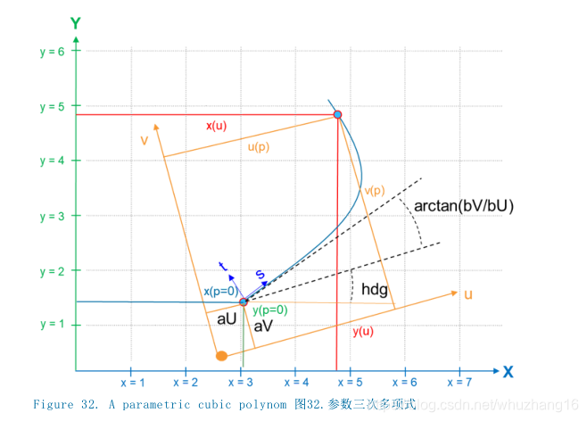
As shown in Figures 26, 27 and 28, assigning non-zero values to the parameters @aU, @aV, and @bV will cause the shift and rotation of the s/t coordinate system.

After defining the point on the curve for the known parameter p, consider the displacement relative to the parameters @aU, @aV, @bU, @bV, starting coordinates (@x,@y) and starting direction @hdg Under the premise of and direction, the u value and v value will be converted into the value in the x/y coordinate system.

It should be noted here that the actual length of the arc between the starting point (@x,@y) in the interpolation parameter p and the <geometry> element and the point (x(p), y(p)) related to the parameter p is nonlinear relationship. Generally speaking, only the start and end parameters p=0 and p=@length (option @pRange=arcLength) are consistent with the actual length of the arc.

In OpenDRIVE, the parametric cubic curve is represented by the <paramPoly3> element in the <geometry> element.

XML example

<planView>
<geometry
s="0.000000000000e+00"
x="6.804539427645e+05"
y="5.422483642942e+06"
hdg="5.287405485081e+00"
length="6.565893957370e+01">
<paramPoly3
aU="0.000000000000e+00"
bU="1.000000000000e+00"
cU="-4.666602734948e-09"
dU="-2.629787927644e-08"
aV="0.000000000000e+00"
bV="1.665334536938e-16"
cV="-1.987729787588e-04"
dV="-1.317158625579e-09"
pRange="arcLength">
</paramPoly3>
</geometry>
</planView>

The following rules apply to parametric cubic curves:
If the starting point of the local u/v coordinate system is consistent with the s/t coordinate system, then the polynomial parameter coefficient is @aU=@aV=@bV=0.

If @pRange="arcLength", then p can be assigned a value in the range of [0, @length from <geometry>].
If @pRange="normalized", then p can be assigned a value in the range [0, 1].
The polynomial parameters aU, bU and aV should be 0 to ensure the smoothness of the reference line.