Machine learning-dimensionality reduction algorithm LDA

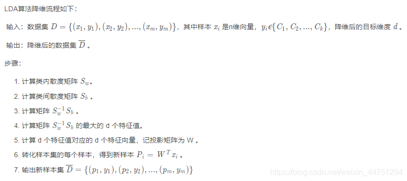
Main process:

Reference articles in the theoretical part:
1. Summary of dimensionality reduction of LDA and PCA
2. Detailed explanation of covariance and covariance matrix
3. Expected value, mean vector and covariance matrix
4. How to calculate mathematical expectation

The following is the use of linear discriminant analysis to complete the dimensionality reduction task on a classic "iris" data set.

The data set contains 3 types of basic data of 150 iris flowers, including 50 data for each of 3 types of Iris iris, color-changing iris, and virginia iris, including 4 characteristics of sepal length, sepal width, petal length, and petal width.

1. Data set processing

# 自己来定义列名，首先读取数据集
feature_dict = {
    
    i:label for i,label in zip(
                range(4),
                  ('sepal length in cm',
                  'sepal width in cm',
                  'petal length in cm',
                  'petal width in cm', ))}

label_dict = {
    
    i:label for i,label in zip(
                range(1,4),
                  ('Setosa',
                  'Versicolor',
                  'Virginica'
                 ))}
import pandas as pd
# 数据读取，大家也可以先下载下来直接读取
df = pd.io.parsers.read_csv(
    filepath_or_buffer='https://archive.ics.uci.edu/ml/machine-learning-databases/iris/iris.data',
    header=None,
    sep=',',
    )
# 指定列名
df.columns = [l for i,l in sorted(feature_dict.items())] + ['class label']

df.head()

	sepal length in cm	sepal width in cm	petal length in cm	petal width in cm	class label
0	5.1	3.5	1.4	0.2	Iris-silky
1	4.9	3.0	1.4	0.2	Iris-silky
2	4.7	3.2	1.3	0.2	Iris-silky
3	4.6	3.1	1.5	0.2	Iris-silky
4	5.0	3.6	1.4	0.2	Iris-silky

Since the features are already numeric data, no additional processing is needed, but a label needs to be converted:

from sklearn.preprocessing import LabelEncoder

X = df[['sepal length in cm','sepal width in cm','petal length in cm','petal width in cm']].values
y = df['class label'].values

# 制作标签{1: 'Setosa', 2: 'Versicolor', 3:'Virginica'}
enc = LabelEncoder()
label_encoder = enc.fit(y)
y = label_encoder.transform(y) + 1

2. Mean vectors in different feature dimensions

In the calculation process, the distance needs to be judged based on the mean value. Therefore, the mean value of each feature in the data must be calculated first, that is, the mean value of each feature of each flower is calculated separately

import numpy as np
#设置小数点的位数
np.set_printoptions(precision=4) 
#这里会保存所有的均值
mean_vectors = []
# 要计算3个类别
for cl in range(1,4):
    # 求当前类别各个特征均值
    mean_vectors.append(np.mean(X[y==cl], axis=0))
    print('均值类别 %s: %s\n' %(cl, mean_vectors[cl-1]))

均值类别 1: [5.006 3.418 1.464 0.244]

均值类别 2: [5.936 2.77  4.26  1.326]

均值类别 3: [6.588 2.974 5.552 2.026]

3. Within-class walking matrix and between-class walking matrix

Next, calculate the within-class walk matrix:

# 原始数据中有4个特征
S_W = np.zeros((4,4))
# 要考虑不同类别，自己算自己的
for cl,mv in zip(range(1,4), mean_vectors):
    class_sc_mat = np.zeros((4,4))    
    # 选中属于当前类别的数据
    for row in X[y == cl]:
        # 这里相当于对各个特征分别进行计算，用矩阵的形式
        row, mv = row.reshape(4,1), mv.reshape(4,1)
        # 跟公式一样
        class_sc_mat += (row-mv).dot((row-mv).T)
    S_W += class_sc_mat                             
print('类内散布矩阵:\n', S_W)

类内散布矩阵:
 [[38.9562 13.683  24.614   5.6556]
 [13.683  17.035   8.12    4.9132]
 [24.614   8.12   27.22    6.2536]
 [ 5.6556  4.9132  6.2536  6.1756]]

Next, calculate the inter-class walk matrix:

# 全局均值
overall_mean = np.mean(X, axis=0)
# 构建类间散布矩阵
S_B = np.zeros((4,4))
# 对各个类别进行计算
for i,mean_vec in enumerate(mean_vectors):  
    #当前类别的样本数
    n = X[y==i+1,:].shape[0]
    mean_vec = mean_vec.reshape(4,1) 
    overall_mean = overall_mean.reshape(4,1) 
    # 如上述公式进行计算
    S_B += n * (mean_vec - overall_mean).dot((mean_vec - overall_mean).T)

print('类间散布矩阵:\n', S_B)

类间散布矩阵:
 [[ 63.2121 -19.534  165.1647  71.3631]
 [-19.534   10.9776 -56.0552 -22.4924]
 [165.1647 -56.0552 436.6437 186.9081]
 [ 71.3631 -22.4924 186.9081  80.6041]]

4. Eigenvalues ​​and eigenvectors

After getting the scatter matrix between the class kernels, you need to combine them together, and then solve the eigenvector of the matrix:

#求解矩阵特征值，特征向量
eig_vals, eig_vecs = np.linalg.eig(np.linalg.inv(S_W).dot(S_B))
# 拿到每一个特征值和其所对应的特征向量
for i in range(len(eig_vals)):
    eigvec_sc = eig_vecs[:,i].reshape(4,1)   
    print('\n特征向量 {}: \n{}'.format(i+1, eigvec_sc.real))
    print('特征值 {:}: {:.2e}'.format(i+1, eig_vals[i].real))

特征向量 1: 
[[-0.2049]
 [-0.3871]
 [ 0.5465]
 [ 0.7138]]
特征值 1: 3.23e+01

特征向量 2: 
[[-0.009 ]
 [-0.589 ]
 [ 0.2543]
 [-0.767 ]]
特征值 2: 2.78e-01

特征向量 3: 
[[-0.8844]
 [ 0.2854]
 [ 0.258 ]
 [ 0.2643]]
特征值 3: 3.42e-15

特征向量 4: 
[[-0.2234]
 [-0.2523]
 [-0.326 ]
 [ 0.8833]]
特征值 4: 1.15e-14

The output results get 4 eigenvalues ​​and their corresponding eigenvectors. It is troublesome to observe the eigenvectors directly, because the projection direction is difficult to understand in high dimensions.

• Feature vector: indicates the mapping direction
• Eigenvalue: the importance of the eigenvector

#特征值和特征向量配对
eig_pairs = [(np.abs(eig_vals[i]), eig_vecs[:,i]) for i in range(len(eig_vals))]

# 按特征值大小进行排序
eig_pairs = sorted(eig_pairs, key=lambda k: k[0], reverse=True)

print('特征值排序结果:\n')
for i in eig_pairs:
    print(i[0])

特征值排序结果:

32.27195779972981
0.27756686384003953
1.1483362279322388e-14
3.422458920849769e-15

print('特征值占总体百分比:\n')
eigv_sum = sum(eig_vals)
for i,j in enumerate(eig_pairs):
    print('特征值 {0:}: {1:.2%}'.format(i+1, (j[0]/eigv_sum).real))

特征值占总体百分比:

特征值 1: 99.15%
特征值 2: 0.85%
特征值 3: 0.00%
特征值 4: 0.00%

Select the first two-dimensional features, which means that the feature data can be reduced to two or even one dimension, but there is no need to reduce it to three dimensions.

Therefore, if you choose to reduce the data to two dimensions, you only need to select the feature vector corresponding to feature value 1 and feature value 2. The first two feature vectors will be spliced ​​together below.

W = np.hstack((eig_pairs[0][1].reshape(4,1), eig_pairs[1][1].reshape(4,1)))
print('矩阵W:\n', W.real)

矩阵W:
 [[-0.2049 -0.009 ]
 [-0.3871 -0.589 ]
 [ 0.5465  0.2543]
 [ 0.7138 -0.767 ]]

The above matrix w is the desired projection direction, and it only needs to be combined with the original data to get the dimensionality reduction result

# 执行降维操作
X_lda = X.dot(W)
X_lda.shape

(150, 2)

It can be seen that the data dimension has been reduced from the original (150,4) to (150,2), and the task of dimensionality reduction has been completed.

5. Visual display

Visual display of raw data

from matplotlib import pyplot as plt
# 可视化展示
def plot_step_lda():

    ax = plt.subplot(111)
    for label,marker,color in zip(
        range(1,4),('^', 's', 'o'),('blue', 'red', 'green')):

        plt.scatter(x=X[:,0].real[y == label],
                y=X[:,1].real[y == label],
                marker=marker,
                color=color,
                alpha=0.5,
                label=label_dict[label]
                )

    plt.xlabel('X[0]')
    plt.ylabel('X[1]')

    leg = plt.legend(loc='upper right', fancybox=True)
    leg.get_frame().set_alpha(0.5)
    plt.title('Original data')

    # 把边边角角隐藏起来
    plt.tick_params(axis="both", which="both", bottom="off", top="off",  
            labelbottom="on", left="off", right="off", labelleft="on")

    # 为了看的清晰些，尽量简洁
    ax.spines["top"].set_visible(False)  
    ax.spines["right"].set_visible(False)
    ax.spines["bottom"].set_visible(False)
    ax.spines["left"].set_visible(False)    

    plt.grid()
    plt.tight_layout
    plt.show()

plot_step_lda()

Visual display of data after dimensionality reduction

from matplotlib import pyplot as plt
# 可视化展示
def plot_step_lda():

    ax = plt.subplot(111)
    for label,marker,color in zip(
        range(1,4),('^', 's', 'o'),('blue', 'red', 'green')):

        plt.scatter(x=X_lda[:,0].real[y == label],
                y=X_lda[:,1].real[y == label],
                marker=marker,
                color=color,
                alpha=0.5,
                label=label_dict[label]
                )

    plt.xlabel('LD1')
    plt.ylabel('LD2')

    leg = plt.legend(loc='upper right', fancybox=True)
    leg.get_frame().set_alpha(0.5)
    plt.title('LDA on iris')

    # 把边边角角隐藏起来
    plt.tick_params(axis="both", which="both", bottom="off", top="off",  
            labelbottom="on", left="off", right="off", labelleft="on")

    # 为了看的清晰些，尽量简洁
    ax.spines["top"].set_visible(False)  
    ax.spines["right"].set_visible(False)
    ax.spines["bottom"].set_visible(False)
    ax.spines["left"].set_visible(False)    

    plt.grid()
    plt.tight_layout
    plt.show()

plot_step_lda()

Use the linear discriminant analysis called in the sklearn toolkit to reduce dimensionality

from sklearn.discriminant_analysis import LinearDiscriminantAnalysis as LDA

# LDA
sklearn_lda = LDA(n_components=2)
X_lda_sklearn = sklearn_lda.fit_transform(X, y)

def plot_scikit_lda(X, title):

    ax = plt.subplot(111)
    for label,marker,color in zip(
        range(1,4),('^', 's', 'o'),('blue', 'red', 'green')):

        plt.scatter(x=X[:,0][y == label],
                    y=X[:,1][y == label] * -1, # flip the figure
                    marker=marker,
                    color=color,
                    alpha=0.5,
                    label=label_dict[label])

    plt.xlabel('LD1')
    plt.ylabel('LD2')

    leg = plt.legend(loc='upper right', fancybox=True)
    leg.get_frame().set_alpha(0.5)
    plt.title(title)

    # hide axis ticks
    plt.tick_params(axis="both", which="both", bottom="off", top="off",  
            labelbottom="on", left="off", right="off", labelleft="on")

    # remove axis spines
    ax.spines["top"].set_visible(False)  
    ax.spines["right"].set_visible(False)
    ax.spines["bottom"].set_visible(False)
    ax.spines["left"].set_visible(False)    

    plt.grid()
    plt.tight_layout
    plt.show()

plot_scikit_lda(X_lda_sklearn, title='Default LDA via scikit-learn')

It can be seen that the result of step-by-step calculation is consistent with the result after dimensionality reduction using the sklearn toolkit