TensorFlow2.0 commonly used functions

Content source video, video address: here

In March 2019, the beta version of
tensorflow 2.0 was released. In October 2019, tensorflow 2.0 was officially released.
In January 2020, tensorflow 2.1 was released.

• Create a tensor,tf.constant(张量内容, dtype=数据类型[可选])

• The numpydata loaded into tensorthe data type,tf.convert_to_tensor(数据名, dtype=数据类型[可选])

• Create an all- 0in tensor tf.zeros(维度),;

• Create an all- 1in tensor tf.ones(维度),;

• Create a tensor with all specified values tf.fill(维度, 指定值),;

• Generating a normal random number, the default mean 0, standard deviation 1, tf.random.normal(维度, mean=均值, stddev=标准差);

• Generate a truncated normal distribution random number tf.random.truncated_normal(维度, mean=均值, stddev=标准差);
  the value of the random number is $(\mu -2\theta ,\mu +2\theta )$ , the outside will be regenerated;

• Generate uniformly distributed random numbers tf.random.uniform(维度, minval=最小值, maxval=最大值),;

• tensorData type conversion tf.cast(张量名, dtype=数据类型):;

• The minimum value of the tensor element dimensions: tf.reduce_min(张量名, axis=轴), axix=0indicates column, 1indicates the row;
  There are similar: tf.reduce_max, tf.reduce_sum, tf.reduce_meanand the like;

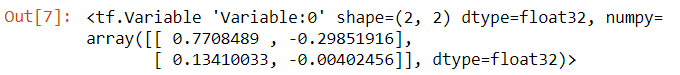
• tf.Variable(初始值)Mark the variable as "trainable", the marked variable will record the gradient information in the backpropagation.
  eg. w = tf.Variable(tf.random.normal([2, 2], mean=0, stddev=1)), that is, the normal distribution randomly initializes the trainable parameters of our defined dimensions w:
  

• Four tf.add(张量1, 张量2)operations: tf.subtract(张量1, 张量2), tf.multiply(张量1, 张量2), , tf.divide(张量1, 张量2), corresponding 维度相同的张量才可进行四则运算arithmetic; .

• tf.square(张量), tf.pow(张量, n次方), tf.sqrt(张量), Corresponding to the square, square root and power;

• Use tf.matmul(矩阵1, 矩阵2)to perform matrix multiplication;

• The pairing, use tf.data.Dataset.from_tensor_slices((输入特征, 标签)), Numpyand Tensorformat of input features and corresponding tags can all use this sentence to read in data.

• The function's derivative operation on the parameters uses the withstructure to record the calculation process to gradientfind the gradient of the tensor.

with tf.GradientTape() as tape:
    若干个计算过程
grad = tape.gradient(函数, 对谁求导)

Case:

with tf.GradientTape() as tape:
    w = tf.Variable(tf.constant(3.0))
    loss = tf.pow(w, 2)
grad = tape.gradient(loss, w)
print(grad) # 6.0

Because the objective function is $Y=w^{2.}$ And the derivative variable of the mark isw, and initialized to a constant3, then the result is6.

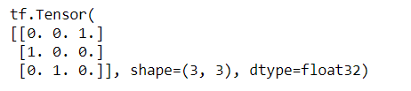
• One-hot encoding means, use tf.one_hot(带转换数据， depth=几分类),
  eg.

datas = tf.constant([2, 0, 1])
classes = 3 # 待分类类别
output = tf.one_hot(datas, depth=classes)
print(output)

• softmaxwhich is:tf.nn.softmax(x)
• Parameter self-updating function,tensor.assign_sub(tensor要自减的内容)

w = tf.Variable(4)
w.assign_sub(2)
print(w) # 2

Similarly, there areassign_add

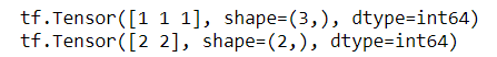
• Returns the maximum subscript of the tensor on the specified axis,tf.argmax(tensor, axis=轴)

a = tf.constant([[1, 2, 3],[4, 5, 6]])
print(tf.argmax(a, axis=0))
print(tf.argmax(a, axis=1))

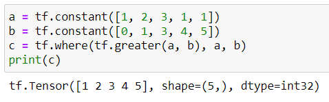
• Conditional statements,tf.where(条件语句, 真返回A, 假返回B)
  
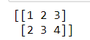
• The two data are superimposed in the vertical direction,np.vstack(数组1, 数组2）

import numpy as np
a = np.array([1, 2, 3])
b = np.array([2, 3, 4])
c = np.vstack((a, b))
print(c)

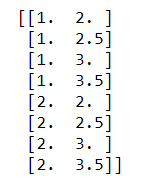
• Grid coordinate point generation,np.mgrid[],.ravel(), np.c_[]

x, y = np.mgrid[1:3:1, 2:4:0.5] # 起始值:结束值:步长
print(x)
print(y)

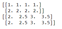
x, y = np.mgrid[1:3:1, 2:4:0.5] # 起始值:结束值:步长
grid = np.c_[x.ravel(), y.ravel()]
print(grid)