I haven't gotten up late at night for more than a year to write a composition, and on rainy nights, I will summarize some ideas.
With a certain bandwidth, the throughput of the network is theoretically not affected by the delay. Although the pipe is a little longer, the cross-sectional area is constant.
However, when you use TCP to verify this conclusion, you often fail to get the results you want:
- A long fat pipe is difficult to be filled by a single TCP connection (a TCP stream is difficult to reach the rated bandwidth in a long fat pipe)!
We do the following topology:
First, I measured the bare bandwidth as a benchmark.
The test receiver is 172.16.0.2, execute iperf -s, and the test sender executes:
iperf -c 172.16.0.2 -i 1 -P 1 -t 2
The results are as follows:
------------------------------------------------------------
Client connecting to 172.16.0.2, TCP port 5001
TCP window size: 3.54 MByte (default)
------------------------------------------------------------
[  3] local 172.16.0.1 port 41364 connected with 172.16.0.2 port 5001
[ ID] Interval       Transfer     Bandwidth
[  3]  0.0- 1.0 sec   129 MBytes  1.09 Gbits/sec
[  3]  1.0- 2.0 sec   119 MBytes   996 Mbits/sec
[  3]  0.0- 2.0 sec   248 MBytes  1.04 Gbits/sec
...
Obviously, the current direct connection bandwidth is 1 Gbits/Sec.
In order to simulate a long fat pipeline with an RTT of 100ms, I used netem to simulate a 100ms delay on the test transmitter (only simulated delay, no packet loss):
tc qdisc add dev enp0s9 root netem delay 100ms limit 10000000
Of course, you can also use netem to simulate a 50ms delay on the test transmitter and test receiver to share the hrtimer overhead.
Execute iperf again, the result is horrible:
------------------------------------------------------------
Client connecting to 172.16.0.2, TCP port 5001
TCP window size:  853 KByte (default)
------------------------------------------------------------
[  3] local 172.16.0.1 port 41368 connected with 172.16.0.2 port 5001
[ ID] Interval       Transfer     Bandwidth
[  3]  0.0- 1.0 sec  2.25 MBytes  18.9 Mbits/sec
[  3]  1.0- 2.0 sec  2.00 MBytes  16.8 Mbits/sec
[  3]  2.0- 3.0 sec  2.00 MBytes  16.8 Mbits/sec
[  3]  3.0- 4.0 sec  2.00 MBytes  16.8 Mbits/sec
[  3]  4.0- 5.0 sec  2.88 MBytes  24.1 Mbits/sec
[  3]  0.0- 5.1 sec  11.1 MBytes  18.3 Mbits/sec
It is totally inconsistent with the theoretical reasoning! The transmission bandwidth of the long fat pipeline does not seem to be free from delay...
So the question is, what on earth is preventing a TCP connection from filling up a long fat pipe?
In order to make things simple and analyzable, I use the simplest Reno algorithm to test:
net.ipv4.tcp_congestion_control = reno
And I turned off Offload features such as TSO/GSO/GRO of the two machines. Under this premise, the story begins.
A common sense that needs to be clear is that the capacity of a long fat pipeline is equal to the product of bandwidth and delay, that is, BDP.
Then, it seems that a single TCP stream fills a long fat pipe with only three conditions:
- In order for the sender to send so much data in BDP, the receiver needs to advertise a window of the size of BDP.
- In order for the sender to have as much data as BDP to send, the sender needs to have a sending buffer as large as BDP.
- In order for the BDP so much data to pass through the long fat pipeline smoothly back-to-back, the network must not be congested (that is, a single-stream exclusive bandwidth is required).
OK, how to meet the above three conditions?
Let me first calculate how big the BDP of a 100ms 1 Gbits/Sec pipeline is. This is easy to calculate. In bytes, its value is:
1024 × 1024 × 1024 8 × 0.1 = 13421772 \dfrac{1024\times 1024\ times 1024}{8}\times 0.1=1342177281024×1024×1024×0.1=1 3 4 2 1 7 7 2 bytes,
about 13MB.
Taking MTU 1500 bytes as an example, I converted BDP into the number of data packets, and its value is:
13421772 1500 = 8947 \dfrac{13421772}{1500}=8947150013421772=8 9 4 7 packets
are 8947 data packets, which is the size of the congestion window required to fill the entire long fat pipeline.
In order to meet the first requirement, I set the receiving buffer of the receiving end to the size of the BDP (it can be larger but not smaller):
net.core.rmem_max = 13420500
net.ipv4.tcp_rmem = 4096 873800 13420500
At the same time, when starting iperf, specify the BDP value as the window. In order to make the receiving window completely unrestricted, I specified the window as 15M instead of just 13M (Linux will also calculate the cost of the skb of the kernel protocol stack. Inside):
iperf -s -w 15m
The prompt shows that the setting is successful:
------------------------------------------------------------
Server listening on TCP port 5001
TCP window size: 25.6 MByte (WARNING: requested 14.3 MByte)
------------------------------------------------------------
OK, let’s look at the sender next, I will also set the send buffer of the sender to the size of BDP:
net.core.wmem_max = 13420500
net.ipv4.tcp_wmem = 4096 873800 13420500
Now I will test it, and the conclusion is still not satisfactory:
...
[  3] 38.0-39.0 sec  18.5 MBytes   155 Mbits/sec
[  3] 39.0-40.0 sec  18.0 MBytes   151 Mbits/sec
[  3] 40.0-41.0 sec  18.9 MBytes   158 Mbits/sec
[  3] 41.0-42.0 sec  18.9 MBytes   158 Mbits/sec
[  3] 42.0-43.0 sec  18.0 MBytes   151 Mbits/sec
[  3] 43.0-44.0 sec  19.1 MBytes   160 Mbits/sec
[  3] 44.0-45.0 sec  18.8 MBytes   158 Mbits/sec
[  3] 45.0-46.0 sec  19.5 MBytes   163 Mbits/sec
[  3] 46.0-47.0 sec  19.6 MBytes   165 Mbits/sec
...
The current limit is no longer the buffer, the current limit is the TCP congestion window! The congestion window seems very reserved and has not been fully opened.
I am so familiar with the TCP Reno congestion control algorithm that I can be sure that such a low bandwidth utilization is the result of its AIMD behavior. It's so easy to handle, I just get around it.
This is a scene without packet loss, so I can manually specify a congestion window by myself. This can be done with only a stap script:
#!/usr/bin/stap -g

%{


#include <linux/skbuff.h>
#include <net/tcp.h>
%}

function alter_cwnd(skk:long, skbb:long)
%{


	struct sock *sk = (struct sock *)STAP_ARG_skk;
	struct sk_buff *skb = (struct sk_buff *)STAP_ARG_skbb;
	struct tcp_sock *tp = tcp_sk(sk);
	struct iphdr *iph;
	struct tcphdr *th;

	if (skb->protocol != htons(ETH_P_IP))
		return;

	th = (struct tcphdr *)skb->data;
	if (ntohs(th->source) == 5001) {


		// 手工将拥塞窗口设置为恒定的BDP包量。
		tp->snd_cwnd = 8947;
	}
%}

probe kernel.function("tcp_ack").return
{


	alter_cwnd($sk, $skb);
}
The following are the test results after specifying the congestion window as BDP:
...
[  3]  0.0- 1.0 sec   124 MBytes  1.04 Gbits/sec
[  3]  1.0- 2.0 sec   116 MBytes   970 Mbits/sec
[  3]  2.0- 3.0 sec   116 MBytes   977 Mbits/sec
[  3]  3.0- 4.0 sec   117 MBytes   979 Mbits/sec
[  3]  4.0- 5.0 sec   116 MBytes   976 Mbits/sec
...
Well, it almost filled the BDP. But the matter is not over.
Now the problem is coming again. I know that TCP Reno is a zigzag upward probe, so the packet loss should be when the BDP is detected, and then the multiplicative window reduction is performed. The average bandwidth should also be at least 50% (for Reno, the reasonable value should be around 75%), why does the test data show that the bandwidth utilization is only about 10%?
Reno will only perform multiplicative window reduction when it detects packet loss. Since the congestion window is far from the maximum capacity allowed by the bandwidth delay, why is there packet loss? What prevents Reno from continuing to visit the window?
No matter if it is the statistics of ifconfig tx/rx on the receiving and sending end or the statistics of tc qdisc, there is no packet loss, and I carefully checked the packet capture at both ends, indeed there are no packets arriving at the receiving end:


The answer is noise loss! That is, link errors, bit inversion, signal decay and so on.
Generally speaking, when the bandwidth utilization rate reaches a certain percentage, there will almost always be accidental, probabilistic noise packet loss. This is very easy to understand. Accidents will always occur, and the probability is high or low. This noise packet loss can be tested by using ping -f on a link with exclusive bandwidth:
# ping -f 172.16.0.2
PING 172.16.0.2 (172.16.0.2) 56(84) bytes of data.
.......^C
--- 172.16.0.2 ping statistics ---
1025 packets transmitted, 1018 received, 0.682927% packet loss, time 14333ms
rtt min/avg/max/mdev = 100.217/102.962/184.080/4.698 ms, pipe 10, ipg/ewma 13.996/104.149 ms
However, even if it is just an accidental packet loss, the blow to TCP Reno is huge. Finally, the window that slowly rises will be immediately reduced to half! This is why it is difficult to climb up the congestion window of TCP connections in the long fat pipeline.
OK, in my test environment, I am sure that the packet loss is caused by noise, because the test TCP connection is completely dedicated to bandwidth without any queuing congestion, so I can block the multiplicative window reduction action, which is not difficult:
#!/usr/bin/stap -g

%{


#include <linux/skbuff.h>
#include <net/tcp.h>
%}

function dump_info(skk:long, skbb:long)
%{


	struct sock *sk = (struct sock *)STAP_ARG_skk;
	struct sk_buff *skb = (struct sk_buff *)STAP_ARG_skbb;
	struct tcp_sock *tp = tcp_sk(sk);
	struct iphdr *iph;
	struct tcphdr *th;

	if (skb->protocol != htons(ETH_P_IP))
		return;

	th = (struct tcphdr *)skb->data;
	if (ntohs(th->source) == 5001) {


		int inflt = tcp_packets_in_flight(tp);
		// 这里打印窗口和inflight值,以观测窗口什么时候能涨到BDP。
		STAP_PRINTF("RTT:%llu  curr cwnd:%d  curr inflight:%d \n", tp->srtt_us/8, tp->snd_cwnd, inflt);
	}
%}

probe kernel.function("tcp_reno_ssthresh").return
{


	// 这里恢复即将要减半的窗口
	$return = $return*2
}

probe kernel.function("tcp_ack")
{


	dump_info($sk, $skb);
}
Now continue to test, let the above script execute first, and then run iperf.
This time I give iperf a long enough execution time, and wait for it to slowly increase the congestion window to BDP:
iperf -c 172.16.0.2 -i 1 -P 1 -t 1500
In a 1 Gbits/Sec long fat pipeline with 100ms RTT, it will be a long process for the congestion window to rise to the size of BDP. Due to the existence of noise and packet loss, the slow start will end soon, ignoring the slow start with a small proportion at the beginning. According to the estimation of adding 1 packet for each RTT window, there are about 10 windows per second, which is 600 per minute, and it takes more than ten minutes for the window to climb to 8000.
…
Go to steam an egg and open another can of Liu Zhi and stinky tofu by the way. Come back and check.
After about 15 minutes, the congestion window no longer increases and stabilizes at 8980. This value is equivalent to the BDP I initially calculated. The following print is the output of the stap script above:
RTT:104118  curr cwnd:8980  curr inflight:8949
RTT:105555  curr cwnd:8980  curr inflight:8828
RTT:107122  curr cwnd:8980  curr inflight:8675
RTT:108641  curr cwnd:8980  curr inflight:8528
The bandwidth at this time is:
...
[  3] 931.0-932.0 sec  121 MBytes   1.02 Gbits/sec
[  3] 932.0-933.0 sec  121 MBytes   1.02 Gbits/sec
[  3] 933.0-934.0 sec  121 MBytes   1.02 Gbits/sec
...
The time required for the window to climb to the BDP is also in line with expectations.
It seems that as long as the multiplicative window reduction of packet loss caused by noise packet loss is ignored, Reno can actually explore the full BDP! The output of 1 Gbits/Sec is so stable, which just shows that the previous packet loss is indeed a noisy packet loss, otherwise the bandwidth would have fallen because of the need to retransmit and queue.
So, the next question is, if TCP has detected the maximum window value, will it continue to probe upwards? In other words, why is the final congestion window stable at 8980 in the above output?
The detail is that when TCP finds that even if it increases the window, it will not bring about an increase in inflight, it will consider it has reached the top and no longer increase the congestion window. See the code snippet below for details:
is_cwnd_limited |= (tcp_packets_in_flight(tp) >= tp->snd_cwnd);
Due to the conservation of data packets, when the value of inflight is less than the congestion window, it means that the quota of the window has not been used up, and there is no need to increase the window. The final maximum value of inflight is limited by the physical limit of the BDP, so it will eventually be stable Value, the congestion window also tends to stabilize.
OK, now you already know how to fill BDP with TCP single stream, this is really difficult!
For Reno, even if I have the ability to ignore noise packet loss (in fact, we cannot distinguish whether the packet loss is caused by noise or congestion), in the large RTT environment of the long fat pipeline, each RTT time will increase the window 1 packet, which is so slow! The "long" of the long fat pipeline can be understood as a long time to increase the window, and the "fat" can be understood as the maximum window of the target is too far away. This understanding is very embarrassing to explain how difficult TCP is in the long fat pipeline!
After Reno, people thought of many optimization methods in an attempt to make TCP's life in the long fat pipeline a little easier, but whether it is BIC or CUBIC, it is a temporary solution, and its ideas are almost the same as Reno.
In the long wait for the last window to climb up, in fact, the noise packet loss is still going on. I just acted as an ostrich hiding its ears and stealing the bell, as nothing happened. However, noise packet loss does not seem to affect the continuous increase in transmission bandwidth, and the result is really like nothing happened.
When I manually specified the window as BDP or when I blocked the window halving effect, due to the SACK enabled, occasional noise packet loss was quickly retransmitted, and the bandwidth remained at the original speed. With the slow increase of the congestion window, the amount of packets sent is also slowly increasing, followed by the slow increase of the iperf measurement transmission rate. After waiting for about 15 minutes, the BDP was filled, and the back-to-back data stream and the back-to-back ACK stream finally connected end to end, and the measurement bandwidth reached the limit. This also fulfilled the requirement at the beginning of this article, that is, let a TCP stream fill a long Fertilizer pipeline.
However, I know very well that in a real environment, first of all, I am not allowed to make logical changes to the protocol stack by stap HOOK. For example, I cannot modify the congestion window of a TCP connection. I can only trust the current congestion control algorithm unconditionally. Secondly, even if I modify the congestion window, for example, I wrote a new congestion control module myself, in which the congestion window was written as a very large value, or I simply blocked the multiplicative window reduction, I would know immediately In reality, this modification will make the situation worse!
I used to be so overwhelmed.
Everything seems to be back to the original point. This is an old problem. I cannot distinguish whether a packet loss is due to noise or congestion. If it is the latter, the window must be multiplicatively reduced.
BBR bypasses this problem. As shown in the previous experimental data, noise packet loss will not affect the actual transmission bandwidth and RTT, but congestion will affect the transmission bandwidth and RTT. BBR calculates the packet sending rate by directly measuring the transmission bandwidth and RTT. After I switched the congestion algorithm to BBR, I tested again with iperf:
root@zhaoya:/home/zhaoya# iperf -c 172.16.0.2  -i 1  -P 1 -t 5
------------------------------------------------------------
Client connecting to 172.16.0.2, TCP port 5001
TCP window size:  853 KByte (default)
------------------------------------------------------------
[  3] local 172.16.0.1 port 41436 connected with 172.16.0.2 port 5001
[ ID] Interval       Transfer     Bandwidth
[  3]  0.0- 1.0 sec  62.4 MBytes   523 Mbits/sec
[  3]  1.0- 2.0 sec   117 MBytes   980 Mbits/sec
[  3]  2.0- 3.0 sec   128 MBytes  1.08 Gbits/sec
[  3]  3.0- 4.0 sec   129 MBytes  1.08 Gbits/sec
[  3]  4.0- 5.0 sec   133 MBytes  1.12 Gbits/sec
[  3]  0.0- 5.0 sec   570 MBytes   955 Mbits/sec
A 5-second test can fill the entire BDP.
Well, the solution to the inefficiency of TCP in the long fat pipeline seems to be very straightforward. Switch to BBR, but is it really that simple?
In addition to bandwidth utilization, congestion control has another important indicator, namely fairness!
Behind the AIMD of Reno/BIC/CUBIC is a mature cybernetic model. Mathematically, it can be proved that Reno (and its descendants BIC, CUBIC) can quickly converge to fairness, but BBR cannot! BBR cannot be mathematically proven to be fair and friendly. This is the essential gap between it and the Reno family congestion control algorithm.
Steal a picture from my previous article:
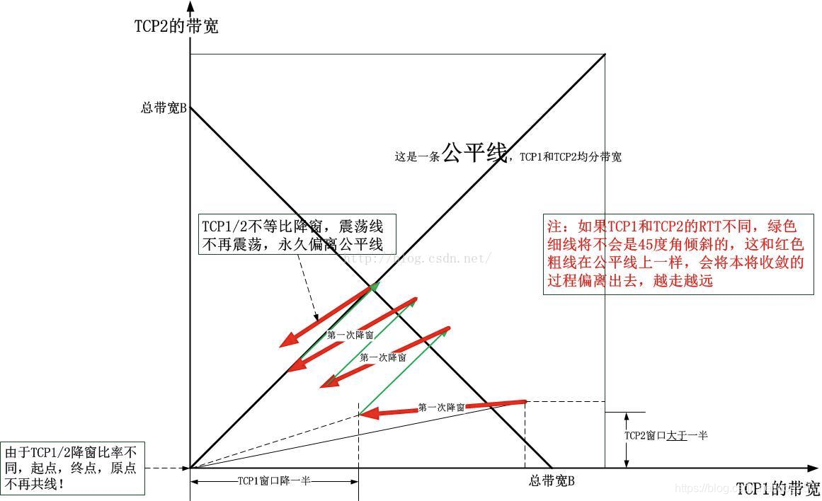
This is an illustration of why the AIMD of the Reno family can converge to fairness. BBR cannot draw such a graph.
When we face a problem, we need to look at history and we need to know how Reno came from. Before the first large-scale network congestion in the 1980s, TCP did not have congestion control. After that, Reno was introduced not for efficiency, but for rapid convergence to fairness when congestion occurred. CUBIC uses the cubic convex-concave curve to optimize the efficiency of window detection on the basis of strict convergence.
No congestion control algorithm is introduced to improve single-stream throughput. On the contrary, if it is to ensure fairness, their effect is often to reduce single-stream throughput. If you want to increase single-stream throughput, you can go back to before 1986.
If you want to maintain efficiency through super-transmission, then you are in line with what everyone expects in the chaotic era without congestion control.
So far, I have not broken away from the ideal test environment I built myself. The performance of TCP in a direct connection environment with exclusive bandwidth is still the same. If it is a public network, the random noise and real congestion in it are more unpredictable. Looking forward to TCP The single-stream throughput climbs to a relatively high level even more can't be expected.
So, how to solve the problem of poor performance of public network TCP in the long fat pipeline?
Cut the long pipes into short ones! It is based on the following knowledge:
- The long pipeline means slow window climbing, slow packet loss perception, and slow packet loss recovery.
- Pipeline fertilizer means that the goal is very ambitious. Combined with the weakness of the pipeline length, it is even more difficult to achieve the goal.
SDWAN can cope with this embarrassment in the long fat pipeline!
There are two ways to split the long fertilizer pipeline:
- TCP proxy mode. Data can be transmitted to remote destinations through multiple transparent proxy relays.
- TCP tunnel mode. The TCP stream with a large delay can be encapsulated in a TCP tunnel with a small delay for relay transmission.
Either way, the path is divided. Since the long path cannot be handled well, the short path should be handled separately. For details, please see:
https://blog.csdn.net/dog250/article/details/83997773
In order to maintain end-to-end transparency, I prefer to use TCP tunnels to split long fat pipes.
Regarding the evaluation of the TCP tunnel itself, I have commented a lot on this topic before:
https://blog.csdn.net/dog250/article/details/81257271
https://blog.csdn.net/dog250/article/details/106955747
In order to get a sense of sight, I will use an experiment to verify the above text.
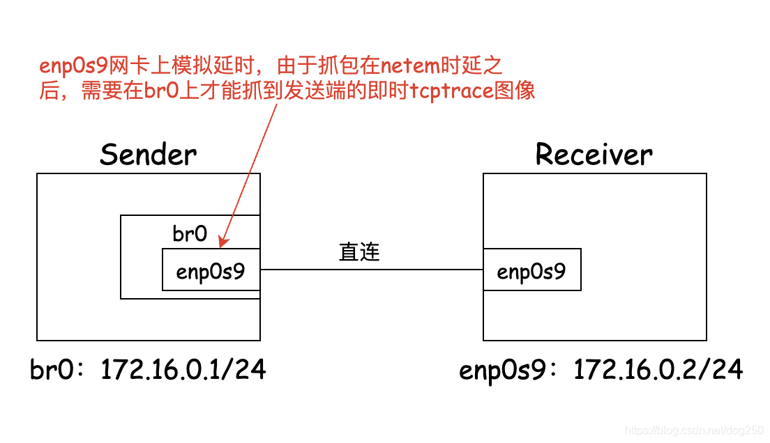
I do the following test topology:

In order to split a simulated long fat pipeline into two sections, I constructed two tunnels and let the tested TCP flow pass through the encapsulation of the two tunnels in turn. In order to build a TCP tunnel, I use the simple ready-made simpletun to complete.
Here is my version of simpletun: https://github.com/marywangran/simpletun
As the example in the README, there is actually no need to configure an IP address for tun0, but the idea of giving an IP address is clearer, so in my experiments, it is all The tun device is assigned an IP address. The following figure is the experimental environment:
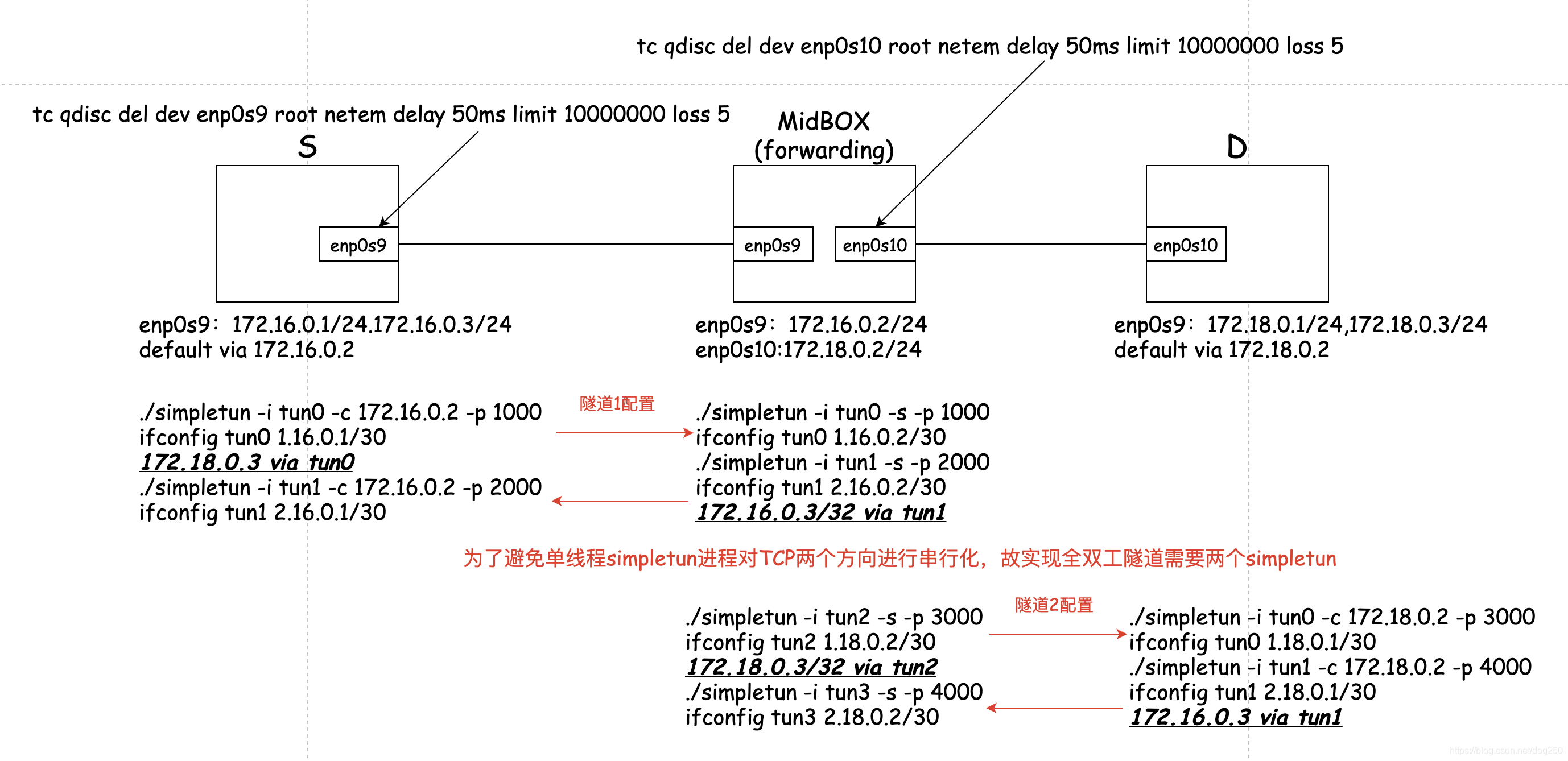
The configuration is written in the figure, the following is the test case:
- case1: Test the throughput of TCP directly through the SD long fat pipeline.
- case2: Test the throughput of TCP from S to D through tunnels T1 and T2.
The following is the test of case1.
Execute iperf -s on D and execute on S:
# 绑定 172.16.0.1
iperf -c 172.18.0.1 -B 172.16.0.1 -i 1  -P 1 -t 15
The results are summarized as follows:
...
[  3]  9.0-10.0 sec  63.6 KBytes   521 Kbits/sec
[  3] 10.0-11.0 sec  63.6 KBytes   521 Kbits/sec
[  3] 11.0-12.0 sec  17.0 KBytes   139 Kbits/sec
[  3] 12.0-13.0 sec  63.6 KBytes   521 Kbits/sec
[  3] 13.0-14.0 sec  63.6 KBytes   521 Kbits/sec
[  3] 14.0-15.0 sec  80.6 KBytes   660 Kbits/sec
[  3]  0.0-15.2 sec  1.27 MBytes   699 Kbits/sec
The following is the test of case2.
Execute iperf -s on D and execute on S:
# 绑定 172.16.0.3
iperf -c 172.18.0.3 -B 172.16.0.3 -i 1  -P 1 -t 15
The results are summarized as follows:
...
[  3]  9.0-10.0 sec  127 KBytes  1.04 Mbits/sec
[  3] 10.0-11.0 sec  445 KBytes  3.65 Mbits/sec
[  3] 11.0-12.0 sec  127 KBytes  1.04 Mbits/sec
[  3] 12.0-13.0 sec  382 KBytes  3.13 Mbits/sec
[  3] 13.0-14.0 sec  127 KBytes  1.04 Mbits/sec
[  3] 14.0-15.0 sec  90.5 KBytes   741 Kbits/sec
[  3]  0.0-15.2 sec  2.14 MBytes  1.18 Mbits/sec
The conclusion is obvious. After the long path is split into the short path, the RTT is obviously smaller, and the packet loss is perceived and the packet loss recovery becomes faster. In addition, a long fat pipeline can be divided and conquered in units of smaller segments, and there is no need to use the same congestion control strategy globally.
Divide and conquer non-homogeneous long fertilizer pipeline, what does it mean?
This means that different TCP tunnel segments can use different congestion control algorithms according to the actual network conditions of the spanned link:
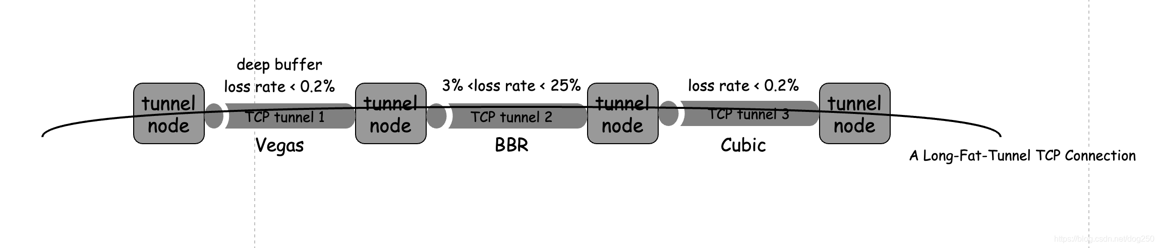
When our wide area network is connected with this or similar Overlay network, we have the ability to define the transmission strategy of each small segment. This fine-grained control capability is exactly what we need.
We need to define a wide area network, we need SDWAN.
Before you know it, it's almost half past eight, and the relationship between people is so strange in this involuntary society! Finally, at the weekend, Xiaoxiao went to cram school again. Basically, the whole family rarely stays awake together in a year.
The leather shoes in Wenzhou, Zhejiang are wet, so they won’t get fat in the rain.