1. Introduction
The selection of prediction model parameters plays a vital role in its generalization ability and prediction accuracy. The parameters of the least squares support vector machine based on the radial basis kernel function mainly involve the penalty factor and the kernel function parameters. The choice of these two parameters will directly affect the learning and generalization ability of the least squares support vector machine. In order to improve the prediction results of the least square support vector machine, the paper uses the gray wolf optimization algorithm to optimize its parameters and establishes a software aging prediction model. Experiments have proved that this model is effective in predicting software aging.
Defects left in the software will cause computer memory leaks, rounding error accumulation, and file locks not released with the long-term continuous operation of the software system, leading to system performance degradation or even crash. The occurrence of these software aging phenomena not only reduces the reliability of the system, but also endangers human life and property safety in serious cases. In order to reduce the harm caused by software aging, it is particularly important to predict the software aging trend and adopt anti-aging strategies to avoid the occurrence of software aging [1].
Many scientific research institutions at home and abroad, such as Bell Labs, IBM, Nanjing University, Wuhan University[2], Xi'an Jiaotong University[3], etc., have conducted in-depth research on software aging and have achieved some results. The main direction of their research is to find the best time to execute the software anti-aging strategy through the prediction of the software aging trend.
This paper takes the Tomcat server as the research object, monitors the operation of Tomcat, collects system performance parameters, and establishes a least squares support vector machine software aging prediction model based on the gray wolf optimization algorithm. Predict the software running status and determine the timing of the software anti-aging strategy.
1 Least Squares
Support Vector Machine Support Vector Machine (SVM) was proposed by Cortes and Vapnik [4]. SVM is based on the VC dimension theory and the principle of structural risk minimization, and can well solve the problems of small samples, nonlinearity, high dimensionality, and local minimums.
When the number of training samples is larger, the SVM solution to the quadratic programming problem is more complicated, and the model training time is too long. Snykens et al. [5] proposed Least Squares Support Vector Machine (LSSVM). On the basis of SVM, equality constraints were used to replace inequality constraints, and the quadratic programming problem was transformed into a linear equation system problem. To a large extent, a large number of complex calculations of SVM are avoided, and the training difficulty is reduced. In recent years, LSSVM has been widely used in regression estimation and nonlinear modeling, and has achieved good prediction results.
In this paper, the radial basis kernel function is used as the kernel function of the LSSVM model. The parameters of the LSSVM algorithm based on the radial basis kernel function mainly involve the penalty factor C and the kernel function parameters. This paper uses the gray wolf optimization algorithm to optimize the parameters of LSSVM.
2 Grey Wolf Optimization Algorithm
In 2014, Mirjalili et al. [6] proposed the Grey Wolf Optimizer (GWO) algorithm. The GWO algorithm found the optimal value by simulating the gray wolf hierarchy and predation strategy in nature. The GWO algorithm has attracted much attention because of its fast convergence and fewer adjustment parameters, and its superiority in solving function optimization problems. This method is superior to particle swarm optimization algorithm, differential evolution algorithm and gravitational search algorithm in terms of global search and convergence, and it is widely used in the fields of feature subset selection and surface wave parameter optimization.
2.1 The principle of
gray wolf optimization algorithm Gray wolf individuals achieve the prosperity and development of the population through collaboration and cooperation, especially in the hunting process, the gray wolf group has a strict pyramid social hierarchy. The wolf with the highest rank is α, and the remaining gray wolves are marked as β, δ, and ω in sequence, and they cooperate to prey.
In the entire group of gray wolves, α wolves play the role of leader in the hunting process, responsible for decision-making during the hunting process and management of the entire wolf pack; β wolves and δ wolves are the sub-adapted groups, they help α wolves to fight the whole wolf The group is managed and has decision-making power during the hunting process; the remaining gray wolf individuals are defined as ω, assisting α, β, and δ to attack their prey.
2.2 Description of gray wolf optimization algorithm
The GWO algorithm imitates the hunting behavior of wolves and divides the entire hunting process into three stages: encircle, hunt, and attack. The process of capturing prey is the process of finding the optimal solution. Assuming that the solution space of gray wolves is V-dimensional, the gray wolf group X is composed of N gray wolf individuals, namely X=[Xi; X2,..., XN]; for gray wolf individuals Xi (1≤i≤N) In other words, its position in the V-dimensional space Xi=[Xi1; Xi2,..., XiV], the distance between the individual position of the gray wolf and the position of the prey is measured by fitness, the smaller the distance, the greater the fitness. The optimization process of GWO algorithm is as follows.
2.2.1 Encirclement
First encircle the prey. In this process, the distance between the prey and the gray wolf is expressed by a mathematical model as follows
: Xp(m) is the position of the prey after the mth iteration, and X(m) is the gray wolf Location, D is the distance between the gray wolf and the prey, A and C are the convergence factor and the swing factor respectively, the calculation formula is:
2.2.2
The optimization process of the hunting GWO algorithm is based on the location of α, β and δ Prey location. ω wolves hunt down their prey under the guidance of α, β, and δ wolves, update their respective positions according to the position of the current best search unit, and re-determine the position of the prey according to the updated α, β, and δ positions. The individual location of the wolves will change with the escape of the prey. The mathematical description of the update process at this stage is:
2.2.3 Attack The
wolves attack and capture the prey to obtain the optimal solution. This process is realized by decrement in formula (2). When 1≤∣A∣, it indicates that the wolves will be closer to the prey, then the wolves will narrow the search range for local search; when 1<∣A∣, the wolves will spread away from the prey, expanding the search range Global search
Second, the source code
tic % 计时
%% 清空环境导入数据
clear
clc
close all
format long
load wndspd
%% GWO-SVR
input_train=[
560.318,1710.53; 562.267,1595.17; 564.511,1479.78; 566.909,1363.74; 569.256,1247.72; 571.847,1131.3; 574.528,1015.33;
673.834,1827.52; 678.13,1597.84; 680.534,1482.11; 683.001,1366.24; 685.534,1250.1; 688.026,1133.91; 690.841,1017.81;
789.313,1830.18; 791.618,1715.56; 796.509,1484.76; 799.097,1368.85; 801.674,1252.76; 804.215,1136.49; 806.928,1020.41;
904.711,1832.73; 907.196,1718.05; 909.807,1603.01; 915.127,1371.43; 917.75,1255.36; 920.417,1139.16; 923.149,1023.09;
1020.18,1835.16; 1022.94,1720.67; 1025.63,1605.48; 1028.4,1489.91; 1033.81,1258.06; 1036.42,1141.89; 1039.11,1025.92;
1135.36,1837.45; 1138.33,1722.94; 1141.35,1607.96; 1144.25,1492.43; 1147.03,1376.63; 1152.23,1144.56; 1154.83,1028.73;
1250.31,1839.19; 1253.44,1725.01; 1256.74,1610.12; 1259.78,1494.74; 1262.67,1379.1; 1265.43,1263.29; 1270.48,1031.58;
1364.32,1840.51; 1367.94,1726.52; 1371.2,1611.99; 1374.43,1496.85; 1377.53,1381.5; 1380.4,1265.81; 1382.89,1150.18;
1477.65,1841.49; 1481.34,1727.86; 1485.07,1613.64; 1488.44,1498.81; 1491.57,1383.71; 1494.47,1268.49; 1497.11,1153.04;
1590.49,1842.51; 1594.53,1729.18; 1598.15,1615.15; 1601.61,1500.72; 1604.72,1385.93; 1607.78,1271.04; 1610.43,1155.93;
1702.82,1843.56; 1706.88,1730.52; 1710.65,1616.79; 1714.29,1502.66; 1717.69,1388.22; 1720.81,1273.68; 1723.77,1158.8;
];
input_test=[558.317,1825.04; 675.909,1712.89; 793.979,1600.35; 912.466,1487.32;
1031.17,1374.03; 1149.79,1260.68; 1268.05,1147.33; 1385.36,1034.68;1499.33,1037.87;1613.11,1040.92;1726.27,1044.19;];
output_train=[
235,175; 235,190; 235,205; 235,220; 235,235; 235,250; 235,265;
250,160; 250,190; 250,205; 250,220; 250,235; 250,250; 250,265;
265,160; 265,175; 265,205; 265,220; 265,235; 265,250; 265,265;
270,160; 270,175; 270,190; 270,220; 270,235; 270,250; 270,265;
285,160; 285,175; 285,190; 285,205; 285,235; 285,250; 285,265;
290,160; 290,175; 290,190; 290,205; 290,220; 290,250; 290,265;
305,160; 305,175; 305,190; 305,205; 305,220; 305,235; 305,265;
320,160; 320,175; 320,190; 320,205; 320,220; 320,235; 320,250;
335,160; 335,175; 335,190; 335,205; 335,220; 335,235; 335,250;
350,160; 350,175; 350,190; 350,205; 350,220; 350,235; 350,250;
365,160; 365,175; 365,190; 365,205; 365,220; 365,235; 365,250;
];
output_test=[235,160; 250,175; 265,190;270,205; 285,220; 290,235; 305,250; 320,265; 335,265; 350,265; 365,265;];
% 生成待回归的数据
x = [0.1,0.1;0.2,0.2;0.3,0.3;0.4,0.4;0.5,0.5;0.6,0.6;0.7,0.7;0.8,0.8;0.9,0.9;1,1];
y = [10,10;20,20;30,30;40,40;50,50;60,60;70,70;80,80;90,90;100,100];
X = input_train;
Y = output_train;
Xt = input_test;
Yt = output_test;
%% 利用灰狼算法选择最佳的SVR参数
SearchAgents_no=60; % 狼群数量
Max_iteration=500; % 最大迭代次数
dim=2; % 此例需要优化两个参数c和g
lb=[0.1,0.1]; % 参数取值下界
ub=[100,100]; % 参数取值上界
Alpha_pos=zeros(1,dim); % 初始化Alpha狼的位置
Alpha_score=inf; % 初始化Alpha狼的目标函数值,change this to -inf for maximization problems
Beta_pos=zeros(1,dim); % 初始化Beta狼的位置
Beta_score=inf; % 初始化Beta狼的目标函数值,change this to -inf for maximization problems
Delta_pos=zeros(1,dim); % 初始化Delta狼的位置
Delta_score=inf; % 初始化Delta狼的目标函数值,change this to -inf for maximization problems
Positions=initialization(SearchAgents_no,dim,ub,lb);
Convergence_curve=zeros(1,Max_iteration);
l=0; % 循环计数器
% %% SVM网络回归预测
% [output_test_pre,acc,~]=svmpredict(output_test',input_test',model_gwo_svr); % SVM模型预测及其精度
% test_pre=mapminmax('reverse',output_test_pre',rule2);
% test_pre = test_pre';
%
% gam = [bestc bestc]; % Regularization parameter
% sig2 =[bestg bestg];
% model = initlssvm(X,Y,type,gam,sig2,kernel); % 模型初始化
% model = trainlssvm(model); % 训练
% Yp = simlssvm(model,Xt); % 回归
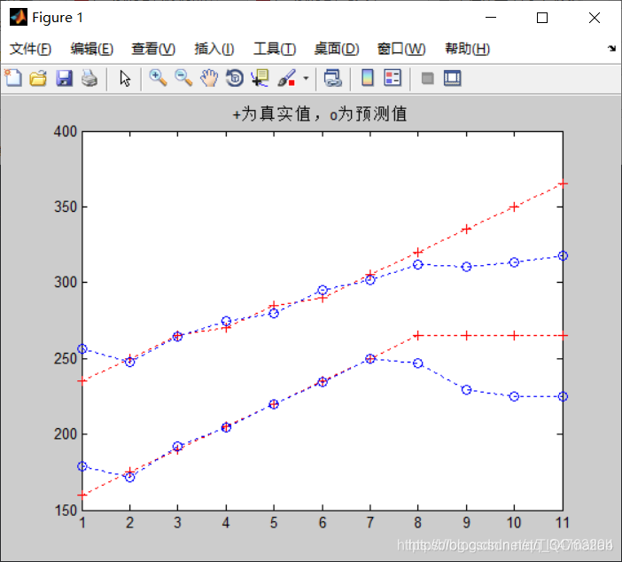
plot(1:length(Yt),Yt,'r+:',1:length(Yp),Yp,'bo:')
title('+为真实值,o为预测值')
% err_pre=wndspd(104:end)-test_pre;
% figure('Name','测试数据残差图')
% set(gcf,'unit','centimeters','position',[0.5,5,30,5])
% plot(err_pre,'*-');
% figure('Name','原始-预测图')
% plot(test_pre,'*r-');hold on;plot(wndspd(104:end),'bo-');
% legend('预测','原始')
% set(gcf,'unit','centimeters','position',[0.5,13,30,5])
%
% result=[wndspd(104:end),test_pre]
%
% MAE=mymae(wndspd(104:end),test_pre)
% MSE=mymse(wndspd(104:end),test_pre)
% MAPE=mymape(wndspd(104:end),test_pre)
%% 显示程序运行时间
toc
Three, running results
Four, remarks
Complete code or writing add QQ912100926 past review
>>>>>>
[Prediction model] lssvm prediction model of particle swarm [Matlab 005]
[lssvm prediction] lssvm prediction of whale optimization algorithm [Matlab 006]
[SVM prediction] SVM prediction model of bat algorithm [Matlab 007]