Introduction to microphone array sound positioning
Generally speaking, sound source localization algorithms based on microphone arrays are divided into three categories: one is based on beamforming; the other is based on high-resolution spectrum estimation; and the third is based on TDOA.
Beamforming
The controllable beamforming technology based on the maximum output power, Beamforming, its basic idea is to form a beam by weighting and summing the signals collected by each array element, guiding the beam by searching the possible position of the sound source, and modifying the weight to make the microphone array The output signal power is the largest. This method can be used both in the time domain and in the frequency domain. Its time shift in the time domain is equivalent to the phase delay in the frequency domain. In the frequency domain processing, a matrix containing self-spectrum and cross-spectrum is first used, which we call the cross-spectral matrix (CSM). At each frequency of interest, the processing of the array signal gives the energy level at each given spatial scanning grid point or each signal direction of arrival (DOA). Therefore, the array represents a sum of responses associated with the sound source distribution. This method is suitable for large microphone arrays and is highly adaptable to the test environment.
The basic working principle diagram of Beamforming:
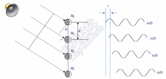
The figure above illustrates: To use the beamforming algorithm, the prerequisite is the far-field sound source (the near-field sound source uses TDOA), so that it can be assumed that the incident sound waves are all parallel; the parallel sound field, if the incident angle is perpendicular to the microphone plane, can be simultaneously If it reaches each microphone, if it is not perpendicular, the phenomenon shown in Figure 1 will appear. There will be a delay when the sound field reaches each microphone. The size of this delay depends on the angle of incidence.
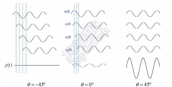
It can be seen from this figure: different incident angles, the superimposed final waveform intensity is not the same. If θ=-45 degrees, there is almost no signal, θ=0 degrees, there is a slight signal, θ=45 degrees, the signal is the strongest. This shows that after the original single microphones without polarity are assembled into an array, the whole array is polarized, and the next polarity diagram can be drawn.
The above figure illustrates: each microphone array is a directional array, and the directivity of this directional array can be simply realized by the time-domain algorithm Delay&Sum, which can control different Delays to achieve different directions. The controllable direction of this directional array is equivalent to giving a spatial filter. The positioning area can be gridded first, and then the time domain delay of each microphone is performed through the Delay time of each grid point, and finally it is summed up. The sound pressure of each grid can be calculated, and the relative sound pressure of each grid can be finally obtained, and a holographic color map of the location of the noise source can be produced.
Based on high resolution spectrum estimation
The methods based on high-resolution spectrum estimation include autoregressive AR model, minimum variance spectrum estimation (MV) and eigenvalue decomposition methods (such as Music algorithm), etc. All these methods calculate the spatial spectrum by obtaining the signal of the microphone array Correlation matrix. In theory, the direction of the sound source can be effectively estimated. In practice, if you want to obtain a more ideal accuracy, you will have to pay a lot of calculation cost and require more assumptions. When the array is large, this spectrum estimation The method has a large amount of calculation, is sensitive to environmental noise, and can easily lead to inaccurate positioning, so it is rarely used in modern large-scale sound source positioning systems.
Sound arrival time difference (TDOA)
Time difference of arrival (TDOA) positioning technology. This type of sound source localization method is generally divided into two steps. First, the time difference of arrival is estimated, and the acoustic delay between elements in the microphone array (TDOA) is obtained from it; The sound arrival time difference is combined with the known spatial position of the microphone array to further determine the position of the sound source.
The figure below explains the basic working principle of TDOA.
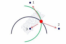
The red dot is the noise source, and the black dot is the microphone. The time delay from the noise source to the two microphones (such as microphone 1, and microphone 3) is a constant. Through this constant, we can draw a green hyperbola from the noise source to microphone 3. , The delay of Mai 2 is another constant. Similarly, we can draw a black curve. The intersection of the two curves is the location of the noise source.
The calculation amount of this method is generally smaller than the previous two methods, which is more conducive to real-time processing, but the positioning accuracy and anti-interference ability are weak. It is suitable for near-field, single sound source, and not repetitive signals, such as voice signals, Microsoft XBOX360 The kinect wheat array (4 one-dimensional arrays with unequal spacing) is a typical application of TDOA algorithm.
Introduction to Positioning System
According to the principle of microphone array sound source positioning, multi-channel noise signals must be collected synchronously for data processing, which must ensure the accuracy of dynamic signal collection. The sound source localization system of its high-tech microphone array mainly uses the NI PXI platform and the cDAQ platform, together with the use of high-performance dynamic data acquisition cards, which can complete accurate acquisition of multi-channel large data volumes.
The software intends to use the SignalPad microphone array module. The specific algorithm used cannot be completely determined at this time. It is necessary to collect the sound characteristics on site, and comprehensively consider the geometrical size, installation location and positioning environment of the array. After a variety of algorithms are comprehensively compared on the spot, the best one is selected.
Microphone array bracket design technology
Only with excellent algorithms, acquisition hardware support is not enough, and excellent microphone holder design technology is also required.
The microphone array is composed of a certain number of microphones arranged in a certain spatial geometric position. Array parameters include geometric parameters such as the number of microphones, the aperture size of the array, the distance between microphone array elements, and the spatial distribution of the microphones; in addition, they also include directivity, beam width, maximum sidelobe level and other characteristic parameters that measure the performance of the array. To design a good array, you need to consider the actual needs and equipment limitations at the same time. In theory, the minimum number of microphones should be used to achieve the best recognition effect.
The number of microphones and the array aperture determine the complexity of an array implementation. The more microphones in the array, the more complicated the wiring method. The array aperture represents the volume occupied by the array in space. The larger the array aperture, the more difficult it is to realize the structure. The number of microphones also affects the array gain. Since the array detects the signal under the background of noise, the array gain is used to describe the improvement of the signal-to-noise ratio provided by the array as a spatial processor. Generally speaking, the number of microphones is proportional to the array gain.
The array should have a better resolution and a larger aperture D; the array should have a higher cut-off frequency and a smaller array spacing. Large apertures and small spacing are contradictory. If they are to be satisfied, only the number of microphones can be increased. In actual use, the design is often weighed against the specific object under test.
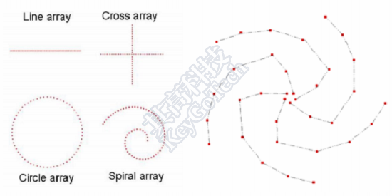
The commonly used arrays are shown in the following figure: they can be divided into regular geometrical arrays and unconventional arrays. Regular geometrical arrays, including linear arrays, cross-shaped arrays, circular arrays, spiral arrays, etc., are all regular geometrical array types, in addition to more complex irregular array types. The two microphones in the irregular array have different position vectors, and the position vectors are linearly independent, which can avoid repeated spatial sampling, suppress aliasing effects, and effectively reduce the appearance of ghosts. However, irregular arrays have higher costs in terms of manufacturing, installation and transportation.
Original website: http://www.keygotech.com/cn/solution/noise-and-vibration/sound-source-localization/noise-source-location-based-on-mic-array