How to FFT (Fast Fourier Transform) to find the amplitude and frequency (super detailed including the derivation process)

How to FFT (Fast Fourier Transform) to find the amplitude and frequency (super detailed including the derivation process)

In order to know this answer, I checked a lot of information and summarized it.

注：本文代码的头文件等如下

import numpy as np
from scipy.fftpack import fft
import matplotlib.pyplot as plt
from matplotlib.pylab import mpl

mpl.rcParams['font.sans-serif'] = ['SimHei']  # 显示中文
mpl.rcParams['axes.unicode_minus'] = False  # 显示负号

1. Beat a chestnut

We set

Sampling frequency is Fs	The highest signal frequency is F	The number of sampling points is N

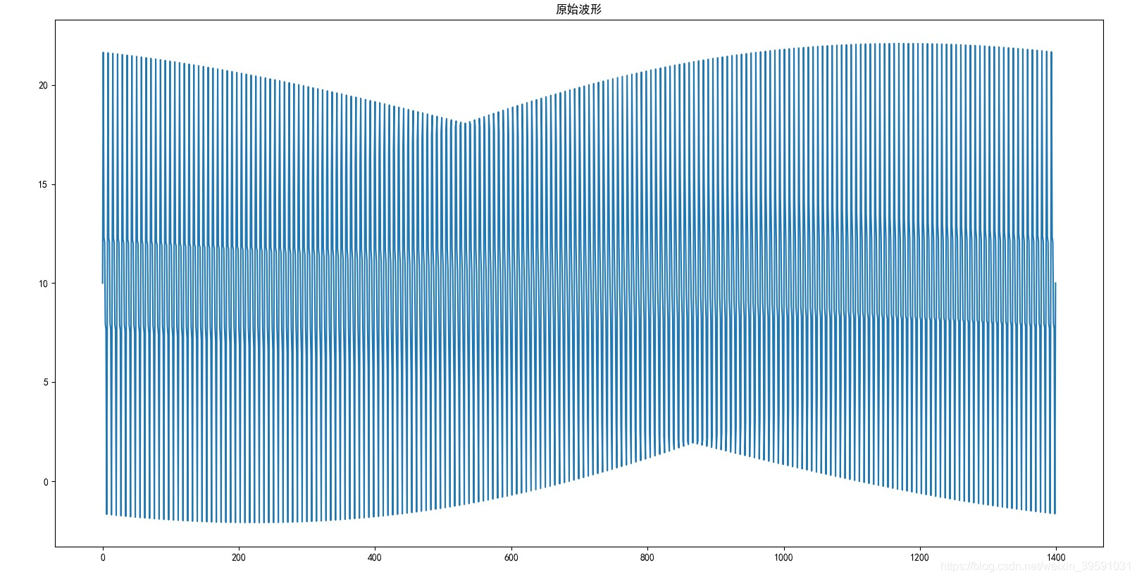
And there is a signal with the following waveform. The signal frequency components 0Hz, 200Hz, 400Hzand 600Hzof the four 标准正弦函数components.

对应完整代码

# 采样点选择1400个，因为设置的信号频率分量最高为600赫兹，根据采样定理知采样频率要大于信号频率2倍，
# 所以这里设置采样频率为1400赫兹（即一秒内有1400个采样点）
N = 1400  # 设置1400个采样点
x = np.linspace(0, 1, N)  # 将0到1平分成1400份

# 设置需要采样的信号，频率分量有0，200，400和600
y = 7 * np.sin(2 * np.pi * 200 * x) + 5 * np.sin(
    2 * np.pi * 400 * x) + 3 * np.sin(2 * np.pi * 600 * x) + 10  # 构造一个演示用的组合信号

plt.plot(x, y)
plt.title('原始波形')
plt.show()

It can be seen that in this example

Sampling frequency Fs	Signal frequency F	Number of sampling points N
1400Hz	600Hz	1,400

So, after the fast Fourier transform (FFT), we will get it N个复数. Every complex value contains 一个特定频率的信息. According to these N complex numbers, we can know the frequencies obtained by splitting the original signal and their amplitude values.

对应代码

fft_y = fft(y)  # 使用快速傅里叶变换，得到的fft_y是长度为N的复数数组

2. Find the amplitude

1. Fast Fourier Transform

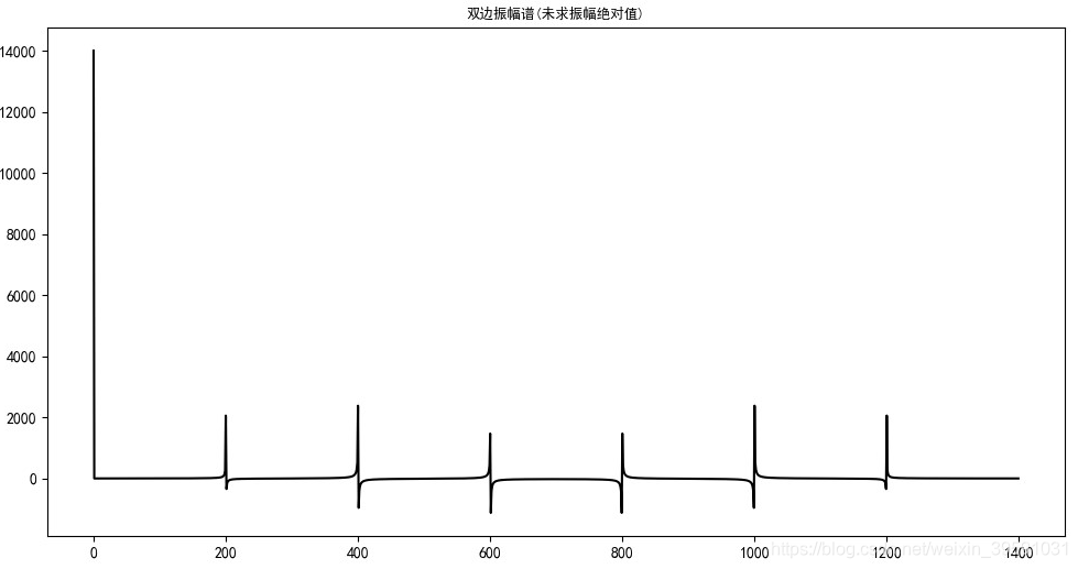
According to the data obtained after the fast Fourier transform, the following irregular graph can be drawn.
(Here, focus on the vertical axis first, and the horizontal axis will be explained in the next section.)

对应完整代码如下

N = 1400  # 设置1400个采样点
x = np.linspace(0, 1, N)  # 将0到1平分成1400份
y = 7 * np.sin(2 * np.pi * 200 * x) + 5 * np.sin(
    2 * np.pi * 400 * x) + 3 * np.sin(2 * np.pi * 600 * x) + 10  # 构造一个演示用的组合信号
fft_y = fft(y)  # 使用快速傅里叶变换，得到的fft_y是长度为N的复数数组

x = np.arange(N)  # 频率个数 （x的取值涉及到横轴的设置，这里暂时忽略，在第二节求频率时讲解）

plt.plot(x, fft_y, 'black')
plt.title('双边振幅谱(未求振幅绝对值)', fontsize=9, color='black')

plt.show()

2. Find the absolute value of a complex number

The graph drawn directly with complex numbers is not what we need. The absolute value (modular length) of all N complex numbers should be found first

abs_y = np.abs(fft_y)  # 取复数的绝对值，即复数的模

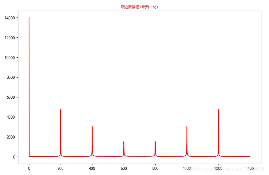
Based on this, the following picture can be drawn

3. Normalization

The figure, the left side of the first value is 从原始信号中提取出来的0Hza corresponding signal strength (signal amplitude), also known 直流分量. Its corresponding signal amplitude is 当前值/FFT的采样点数N, namely

0Hz corresponding amplitude = current value / number of sampling points N

Note:

1. In this example, the corresponding amplitude of the DC component = 14000/1400 = 10
2. The current value is the absolute value (modulo length) obtained from the current complex number

The signal amplitude corresponding to the components other than the DC component 当前值/（采样点数N/2）is:

Amplitude corresponding to other frequencies = current value/(number of sampling points N / 2)

Note:

1. In this example, 200Hz corresponds to amplitude = 5000 / (1400 / 2) ≈ 7.14 (5000 here is the estimated value obtained by looking at the picture, just for example, not necessarily accurate), the other frequencies correspond to the same amplitude algorithm.

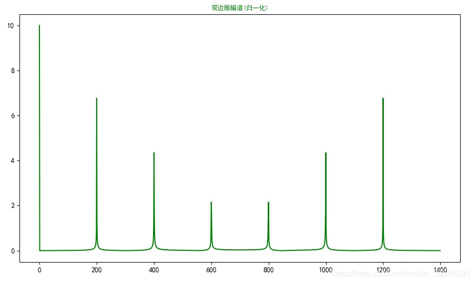
So, after normalization, we get the following figure

对应完整代码

N = 1400  # 设置1400个采样点
x = np.linspace(0, 1, N)  # 将0到1平分成1400份
y = 7 * np.sin(2 * np.pi * 200 * x) + 5 * np.sin(
    2 * np.pi * 400 * x) + 3 * np.sin(2 * np.pi * 600 * x) + 10  # 构造一个演示用的组合信号
fft_y = fft(y)  # 使用快速傅里叶变换，得到的fft_y是长度为N的复数数组

x = np.arange(N)  # 频率个数（x的取值涉及到横轴的设置，这里暂时忽略，在第二节求频率时讲解）

abs_y = np.abs(fft_y)  # 取复数的绝对值，即复数的模
normalization_y = abs_y / (N / 2)  # 归一化处理（双边频谱）
normalization_y[0] /= 2

plt.plot(x, abs_y, 'r')
plt.title('双边振幅谱(归一化)', fontsize=9, color='red')
plt.show()

summary

DC component (0Hz) amplitude	Other frequency amplitude
The absolute value of the complex number obtained by fft / N	The absolute value of the complex number obtained by fft / (N / 2)

Three. Find the frequency

First put a paragraph of text here, which explains the method of finding frequency more vividly.

For example, you have an analog signal with the highest frequency f = 32kHz and a sampling frequency of 64kHz. Perform a 16-point FFT analysis on this signal. The range of the sampling point subscript n is 0, 1, 2, 3, …, 15. Then the analog frequency of 64kHz is divided into 16 parts, each part is 4kHz, this 4kHz is called frequency resolution.
Therefore, in the abscissa of the frequency chart:
n=1 corresponds to f is 4kHz
n=2 corresponds to f is 8kHz
…
n=15 corresponds to f is 60kHz
and the frequency spectrum is symmetrical about n=8, just care about n=0 A spectrum of ~7 is sufficient. Because the highest frequency of the original signal is 32kHz.
(This paragraph is adapted from Reference 1)

1. Frequency formula

Therefore, after knowing the sampling frequency Fs, the actual frequency corresponding to the xth (x starts from 0) complex value after the fast Fourier transform (FFT) is

f (x) = x * (Fs / n)

So, in this example,

The frequency of the 0th point f(0) = 0 * (1400 / 1400) = 0
The frequency of the first point f(0) = 1 * (1400 / 1400) = 1
The frequency of the second point f(0) = 2 * (1400 / 1400) = 2
…
the frequency of the 200th point f(200) = 200 * (1400 / 1400) = 200
…
the frequency of the 1400th point f(200) = 1400 * (1400 / 1400) = 1400
(Because of the coincidence, the frequency corresponding to the x-th point is exactly x)

Now we know why the x-axis coordinate value is set in this way.

2. Remove duplicate values

Only the half of the frequency from 0 to N/2 is valid, and the other half is symmetrical to this half. After removing the duplication, we get the following picture

Corresponding to the complete code:

N = 1400  # 设置1400个采样点
x = np.linspace(0, 1, N)  # 将0到1平分成1400份
y = 7 * np.sin(2 * np.pi * 200 * x) + 5 * np.sin(
    2 * np.pi * 400 * x) + 3 * np.sin(2 * np.pi * 600 * x) + 10  # 构造一个演示用的组合信号
fft_y = fft(y)  # 使用快速傅里叶变换，得到的fft_y是长度为N的复数数组

x = np.arange(N)  # 频率个数（x的取值涉及到横轴的设置，这里暂时忽略，在第二节求频率时讲解）
half_x = x[range(int(N / 2))]  # 取一半区间

abs_y = np.abs(fft_y)  # 取复数的绝对值，即复数的模
normalization_y = abs_y / (N / 2)  # 归一化处理（双边频谱）
normalization_y[0] /= 2
normalization_half_y = normalization_y[range(int(N / 2))]  # 由于对称性，只取一半区间（单边频谱）

plt.plot(half_x, normalization_half_y, 'blue')
plt.title('单边振幅谱(归一化)', fontsize=9, color='blue')
plt.show()

summary

Among the n complex values ​​obtained after FFT, the frequency f(x) corresponding to the xth (x starts from 0) complex value is

f (x) = x * (Fs / n)

Appendix: Complete code

import numpy as np
from scipy.fftpack import fft
import matplotlib.pyplot as plt
from matplotlib.pylab import mpl

mpl.rcParams['font.sans-serif'] = ['SimHei']  # 显示中文
mpl.rcParams['axes.unicode_minus'] = False  # 显示负号

# 采样点选择1400个，因为设置的信号频率分量最高为600赫兹，根据采样定理知采样频率要大于信号频率2倍，
# 所以这里设置采样频率为1400赫兹（即一秒内有1400个采样点，一样意思的）
N = 1400
x = np.linspace(0, 1, N)

# 设置需要采样的信号，频率分量有0，200，400和600
y = 7 * np.sin(2 * np.pi * 200 * x) + 5 * np.sin(
    2 * np.pi * 400 * x) + 3 * np.sin(2 * np.pi * 600 * x) + 10

fft_y = fft(y)  # 快速傅里叶变换

x = np.arange(N)  # 频率个数
half_x = x[range(int(N / 2))]   # 取一半区间

angle_y = np.angle(fft_y)       # 取复数的角度

abs_y = np.abs(fft_y)               # 取复数的绝对值，即复数的模(双边频谱)
normalization_y = abs_y / (N / 2)   # 归一化处理（双边频谱）
normalization_y[0] /= 2             # 归一化处理（双边频谱）
normalization_half_y = normalization_y[range(int(N / 2))]  # 由于对称性，只取一半区间（单边频谱）


plt.subplot(231)
plt.plot(x, y)
plt.title('原始波形')

plt.subplot(232)
plt.plot(x, fft_y, 'black')
plt.title('双边振幅谱(未求振幅绝对值)', fontsize=9, color='black')

plt.subplot(233)
plt.plot(x, abs_y, 'r')
plt.title('双边振幅谱(未归一化)', fontsize=9, color='red')

plt.subplot(234)
plt.plot(x, angle_y, 'violet')
plt.title('双边相位谱(未归一化)', fontsize=9, color='violet')

plt.subplot(235)
plt.plot(x, normalization_y, 'g')
plt.title('双边振幅谱(归一化)', fontsize=9, color='green')

plt.subplot(236)
plt.plot(half_x, normalization_half_y, 'blue')
plt.title('单边振幅谱(归一化)', fontsize=9, color='blue')

plt.show()

Appendix: Derivation Process

For details, see the formula conversion between the circular frequency w and the frequency f in the Fourier transform

Reference materials:

1. Normalized frequency in digital signal processing
2. Use python (scipy and numpy) to implement fast Fourier transform (FFT) the most detailed tutorial
3. After getting the complex number after FFT, how to find the frequency based on this complex number?
4. FFT frequency and amplitude determination
5. In the Fourier transform, the formula conversion between the circular frequency w and the frequency f