The purpose of communication is to instantly and reliably (and sometimes secretly) deliver messages that the other party does not know. When there is interference in the channel, the sent message may be wrong. In digital communication, error correction code technology is usually used for error control, which can improve the reliability of data transmission.
The BCH code is a widely used block code that can correct multiple errors and has excellent error correction performance. This article conducts an in-depth analysis of the principle of BCH code, and introduces the principle of BCH codec. It focuses on the calculation method of BCH encoding and decoding and the performance analysis of BCH encoding. Finally, this article uses MATLAB to write the corresponding BCH codec code for simulation and bit error rate analysis, and build a BCH module in Simulink for bit error rate statistical analysis. The research results made in this paper have certain scientific research value and provide a good theoretical basis for the further research of BCH or the realization of hardware system.
1.1 Research background of this subject
When a digital signal is transmitted in a transmission system, it is inevitably interfered by various factors, so that the digital signal arriving at the receiving end will be mixed with noise, which will lead to erroneous judgments. In order to fight the interference, the error control technology of the error correction code must be used.
There are the following categories of error correction codes:
·According to the different processing methods of the information sequence, it is divided into two categories: block codes and convolutional codes. According to the structural characteristics of the codes, the block codes can be divided into cyclic codes and acyclic codes.
·Divided into linear code and non-linear code according to the relationship between information bit and check bit.
·According to the applicable error type, it is divided into two types: random error code and error burst error code. There are also random error/burst error codes in between.
·According to the theory of code construction, there are algebra, geometry, arithmetic, combination codes, etc.
In addition to the above classification, there are as many classification methods as there are perspectives to observe the problem. For example, according to the value of each symbol, it can be divided into binary code and multi-system code; according to the relationship between code words, there are cyclic codes and non-cyclic codes; different classification methods are only grasped from different angles. Categorizing a certain characteristic of the code alone does not mean that a certain code is all the characteristics. For example, a certain linear code may be block code, cyclic code, error burst error code, algebraic code, and binary code at the same time.
1.2 Linear block codes and cyclic codes
Linear block code is the most important type of block code, represented by (n, k), where n is the code length, k is the number of information bits, nk=r is the number of check bits, and binary (n, k) is linear The block code can be defined as a k-dimensional subspace in the n-dimensional linear space Vn in the GF(2) domain.
There are three important parameters in the linear block code, namely the code rate, the Hamming distance and the Hamming weight of the code. The code rate R=k/n, it illustrates the effectiveness of the block code to transmit information. The Hamming distance of a code refers to the number of different code elements on the corresponding bits of two code words, referred to as distance. Hamming weight refers to the number of non-zero symbols in a codeword, referred to as weight. In the (n, k) linear block code, the minimum distance between any two codewords is called the minimum distance d0. Since the linear block code is a group code, it can be known from the closeness of the group code that if the codewords C1 and C2 are codewords of the (n, k) code, then C1+C2 must also be another codeword of the block code. It can be seen that the minimum distance of the (n, k) linear block code is equal to the minimum weight of the non-zero codeword. The minimum distance d. It directly determines the error detection and correction capabilities of the code in theory.
Cyclic codes are the most important subclass of linear block codes. Its algebraic structure is relatively clear. Compared with other codes, the codec is simple and easy to implement. Therefore, cyclic codes are widely used in error control systems. BCH codes are A very important class of cyclic codes.
In the n-dimensional linear space gas on GF(2), if it is a k-dimensional subspace, for any, there is a cyclic code.
The error correction capability of the cyclic code derived from the coding theory is only a theoretical value, and whether this theoretical value can be achieved in reality is also related to the decoding method used. A good decoding method should not only enable the error correction capability to reach the theoretical limit, but also achieve high speed and low cost, because speed and cost sometimes become the decisive factor for the practicality of a certain code.
Decoding circuits are usually much more complicated than coding circuits. Therefore, we say that the complexity of theory is often reflected in the encoding, and the complexity of engineering is often reflected in the decoding. From the degree of quantization of the input signal, decoding can be divided into hard decision decoding (BSC channel) and soft decision decoding (DMC channel).
Since soft decision uses a quantization level greater than 2, it can make full use of the information contained in the received signal. Compared with hard decision, it can have a coding gain of 2dB in the AWGN channel and 10-2-10 coin error rate range. , Therefore represents the development direction of decoding. From the error control method, decoding can be divided into two types: error correction and error detection. The error correction decoder always has an output, but there are two possibilities: First, the number of errors in the received code is within the error correction capability, and the decoder determines that it is correct. The second is that the number of errors exceeds the error correction capability, and what the decoder determines to be correct is actually wrong. Since it is difficult to judge whether the number of errors exceeds the error correction capability, the error correction decoder cannot guarantee the complete reliability of the output data, so the error correction decoder is often used in forward error correction (FEC) of digital voice, image, and video signals.
1.3 Research and application of BCH coding
The BCH code was proposed by Hokkungum in 1959 and Bo and Ray Chadhury in 1960 and named after these three discoverers. BCH codes are a good class of linear error correction codes discovered so far. Its error correction ability is very strong, especially under the condition of medium and short code length, the performance of the BCH code is close to the theoretical best value, and the structure is convenient and the coding is simple. In particular, it has a strict algebraic structure and plays an important role in algebraic coding theory. The BCH code is a linear block code that has been studied in detail, well understood, and achieved the most results so far.
In 1960, Peterson solved the decoding algorithm of binary BCH code theoretically, laying the theoretical foundation of BCH code decoding. Later, Greenstein and Ziller generalized it to multi-system. In 1966, Berlicamp used an iterative algorithm to translate the BCH code, which greatly accelerated the decoding speed and actually solved the decoding problem of the BCH code. Because the BCH code has excellent performance, simple structure, and not too complicated encoding and decoding equipment, it is welcomed by engineers and technicians in actual use, and it is currently one of the most widely used code types.
In the British analog mobile communication system, the base station uses the BCH (40, 28) code capable of correcting 2-bit random errors, and the mobile station uses the BCH (48, 36) code that can correct 2-bit random errors; In the call system, the BCH (31, 21) code plus a parity bit is used as the FEC method; in the video coding protocol H.261 and H.263, the BCH (511, 493) code is used for video error correction.
Chapter 3 Introduction to BCH Code Theory
3.1 Introduction to BCH code
BCH codes are an important subclass of cyclic codes, which have the ability to correct multiple errors. BCH codes have strict algebraic theory and are currently the most thoroughly studied type of codes. There is a close relationship between its generator polynomial and the minimum code distance. People can easily construct BCH codes according to the required error correction ability t, and their decoders are also easy to implement. They are the most commonly used linear block codes. One type of code.
3.1.1 Galois Field
The most basic and important fields in the coding principle are the binary Galois field GF(2) and the binary extended field GF(2m). The set of finite positive numbers F={0,1,2,3,...,q-1} (q is a prime number) forms a q-order finite field under the modulo q addition and modulo q multiplication operations, also known as Galois ) Domain, denoted as GF(q). When q=2, it is the binary field GF(2).
The operation defined in the finite field satisfies the closedness, that is, the operation ⊙ of any two elements A and B on the finite field GF(q) satisfies: A⊙B∈GF(q).
If p is a prime number, m is a positive integer, the smallest subdomain of GF(2m) is GF(p), and p is called the feature of GF(2m). In the Galois field with feature 2, any field element B has -B=B.
Let B be any element on GF(q), then B=Bq.
Each Galois field GF(q) contains at least one primitive element α, and any field element on GF(q) except zero can be expressed as a power of the primitive element.
Any finite field can be composed of a primitive polynomial, and any polynomial in the finite field modulates the primitive polynomial to obtain a polynomial whose degree is lower than the degree of the primitive polynomial, that is, the element of the finite field.
·Addition
The addition operation of the field elements is converted into the corresponding m-1 degree polynomial coefficients (m multiple vectors) according to the field element table. The addition of two field elements is equivalent to the addition of the same degree coefficient modulo 2 of two m-1 degree polynomials, that is, the exclusive OR operation.
·Multiplication
There are three ways to achieve multiplication:
The first is to directly shift the polynomial coefficients corresponding to the field elements, such as a×b, as long as the power corresponding to b is found, assuming it is x, shift a to the left x times, and judge the high value of the value before shifting each time to the left Whether it is 1, if it is 1, add the original polynomial divided by the higher power after shifting;
The second method is to start from the high bit of b. If b7=1, move a to the left 7 times, if b6=1, move the result to the left and then move it to the left 6 times.
The third method is to directly add the exponents of the domain elements to modulo 2m-1. The third method is used here.
·Modulo calculation
Because the conversion of 2^m-1 into binary numbers is always all 1, so according to this feature, you can use the following method to find the modulus. The number in binary form is divided into m bits from the low order, and the high order is less than m bits filled with 0. Then every time a 1 appears in the high-order segment, subtract 1 from the high-order segment, and then add 1 to the low-order segment, so that the loop operation until the high-order segment becomes all 0s.


3.3 Introduction to BCH decoding theory
BCH code decoding can be divided into time domain decoding and frequency domain decoding.
Frequency-domain decoding treats the codeword as a time-domain digital sequence, transforms it into the frequency domain by discrete Fourier transform (DFT) in the finite domain, and then uses its frequency domain characteristics to decode. In this way, the key equation indicating the position of the error is solved through the operation of the frequency-domain syndrome, and then the time-domain error correction signal is restored through the discrete Fourier inverse change.
Time domain decoding treats the codeword as a signal sequence on the time axis, and uses the algebraic structure of the code for decoding. Because the finite-domain discrete Fourier transform increases the complexity, the realization of frequency-domain decoding is generally more complicated than that of time-domain decoding. Therefore, the frequency-domain decoding using fast Fourier transform (FFT) can only be used in certain special cases. Code length (for example, n is equal to a power of 2) decoding is better than time domain decoding, and in general, time domain decoding is the most widely used. The basic structure of the BCH decoder is as follows:
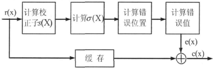
Figure 3-1 Basic structure block diagram of BCH decoder
Usually, we design an algorithm in MATLAB in three steps:
·STEP1: Calculate the syndrome S from the received R(x);
·STEP2: The error pattern E(x) is obtained from the syndrome;
· STEP3 : Get the estimated codeword c(x) from R(x)-E(x).
5.2 System simulation of BCH encoding
We write MATLAB code based on the previous theoretical analysis. Here, we perform BCH encoding of two parameters (511,493)(4095,4035) according to requirements, and the MATLAB encoding function is as follows:
function code=bchencoder(data,genpoly,n,k);
bb=zeros(1,n-k);
for i=k:-1:1
feedback = xor(data(i), bb(n-k));
if feedback~=0
for j=n-k:-1:2
if genpoly(n-k-j+2)~=0
bb (j) = xor (bb (j-1), feedback);
else
bb(j)=bb(j-1);
end
end
bb(1)=feedback;
else
for j=n-k:-1:2
bb(j)=bb(j-1);
end
bb(1)=feedback;
end
end
code=[bb,data];
We call it at the top level, the calling process is as follows:
for j=1:nwords
encoded_data((j-1)*n+1:(j-1)*n+n)=bchencoder(message((j-1)*k+1:(j-1)*k+k),genpoly,n,k);
end
The input information is:
………… 1 1 0 1 1 0 0 1 1 1 …………………………
After BCH coding, BCH coding information is obtained:
………… 1 1 0 0 0 1 0 0 1 0 …………………………
5.3 System simulation of BCH decoding
In the decoding of this system, we will use the widely used "money search" method for decoding. We have briefly introduced the algorithm before. The MATLAB code implementation process is as follows:
lambda_v = zero;
accu_tb=gf(ones(1, t+1), m);
for i=1:n,
lambda_v = lambda * accu_tb ';
accu_tb = accu_tb. * inverse_tb;
if(lambda_v==zero)
error(1,n-i+1)=1;
else
error(1,n-i+1)=0;
end
end
found = find(error(1,:)~=0);
for i=1:length(found)
location=found(i);
if location <= k;
rec_data(n-location+1)=rec_data(n-location+1)+one;
end
end
decoded_data((j-1)*k+1:(j-1)*k+k)=rec_data(n-k+1:n);
We input the signal obtained after encoding into the BCH decoding part, and output the result:
………… 1 1 0 1 1 0 0 1 1 1 …………………………
5.2.4 Performance analysis of BCH encoding and decoding with different parameters
In this chapter, we will focus on the simulation of several BCH codes with different parameters. For the analysis of the system SNR, we mainly adopt: ' semilogy ' for simulation. We simulated (511,493)(4095,4035) respectively, and then did not change the two parameters n, k, and changed its error correction capability to simulate, thereby judging the performance of BCH encoding and decoding.

Figure 5-1 S/N ratio under n= 511,k=493 , t=11 conditions

Figure 5-2 SNR under the condition of n= 4095 , k= 4035 and t=11

Figure 5-3 Performance comparison between BCH encoding and non-encoding (green means failing encoding)
It can be seen from the simulation results that, for BCH codes with the same error correction capability, the performance of the shorter codeword length is better than the longer codeword length, and the average simulation time for a codeword is less. The reason for the analysis is that under the same channel conditions, the probability of each symbol having an error is the same. For a BCH code with a long codeword length, the average number of symbols with errors in each codeword is large, so for BCH codes with the same error correction capability have poor performance with long codeword lengths.
Above we have introduced MATLAB's BCH codec and signal-to-noise ratio analysis in detail. Next, we will perform BCH actual simulation in Siumlink. In this system, we will perform simulation analysis based on BPSK.
The BPSK system without BCH is as follows:
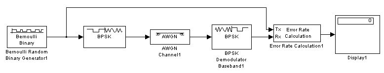
Figure 5-4 BPSK simulation system
The simulation results are as follows:
Add BCH codec, the system is as follows:

Figure 5-5 BCH simulation system
The simulation results are as follows:

As can be seen from the figure above, after adding BCH encoding and decoding, the new performance has been greatly improved.
·Encoding and decoding
clc;
clear;
close all;
m=9;% input parameter 6
k=493;% input parameter 4
snr=1;
n=2^m-1;
period=1000;
nwords = ceil(1000/k);
[genpoly,t] = bchgenpoly(n,k);
simplified = 1;
alpha = gf(2, m);
zero = gf(0, m);
one = gf(1, m);
message=randint(1,nwords*k);
message1=gf(message);
decoded_data=gf(zeros(1,nwords*k));
alpha_tb=gf(zeros(1, 2*t), m);
for i=1:2*t,
alpha_tb(i)=alpha^(2*t-i+1);
end;
%BCH code
for j=1:nwords
encoded_data((j-1)*n+1:(j-1)*n+n)=bchencoder(message((j-1)*k+1:(j-1)*k+k),genpoly, n,k);% from high to low
end
%Add noise
sigma=sqrt(1/(10^(snr/10))/2);
datalength=length(encoded_data);
snum=ceil(datalength/period);
for(i=1:snum-1)
data2((i-1)*period+1:(i-1)*period+period)=encoded_data((i-1)*period+1:(i-1)*period+period)+sigma*randn(1,period);
end
data2((snum-1)*period+1:datalength)=encoded_data((snum-1)*period+1:datalength)+sigma*randn(1,length(encoded_data((snum-1)*period+1:datalength)));
rec_data2=zeros(1,nwords*n);
for i=1:nwords*n
if abs(encoded_data(i)-data2(i))>0.5
rec_data2(i)=xor(encoded_data(i),1);
else
rec_data2(i)=encoded_data(i);
end
end
rec_data2=gf(rec_data2,m);
%BCH decoding
for j=1:nwords
rec_data=rec_data2((j-1)*n+1:(j-1)*n+n);
syndrome=gf(zeros(1, 2*t), m);
for i=1:n,
syndrome=syndrome.*alpha_tb+rec_data(n-i+1);
end;
lambda = gf([1, zeros(1, t)], m);
lambda0 = lambda;
b=gf([0, 1, zeros(1, t)], m);
b2 = gf([0, 0, 1, zeros(1, t)], m);
k1 = 0;
gamma = one;
delta = zero;
syndrome_array = gf(zeros(1, t+1), m);
if(simplified == 1)
for r=1:t,
r1 = 2*t-2*r+2;
r2 = min(r1+t, 2*t);
num = r2-r1+1;
syndrome_array(1: num) = syndrome(r1:r2);
delta = syndrome_array*lambda';
lambda0 = lambda;
lambda = gamma*lambda-delta*b2(2:t+2);
if((delta~= zero) && (k1>=0))
b2(3)=zero;
b2(4:3+t) = lambda0(1:t);
gamma = delta;
k1 = -k1;
else
b2(3:3+t) = b2(1:t+1);
gamma = gamma;
k1 = k1 + 2;
end
joke=1;
end
else
for r=1:2*t,
r1 = 2*t-r+1;
r2 = min(r1+t, 2*t);
num = r2-r1+1;
syndrome_array(1:num) = syndrome(r1:r2);
delta = syndrome_array*lambda';
lambda0 = lambda;
lambda = gamma*lambda-delta*b(1:t+1);
if((delta ~= zero) && (k1>=0))
b(2:2+t)=lambda0;
gamma = delta;
k1 = -k1-1;
else
b (2: 2 + t) = b (1: t + 1);
gamma = gamma;
k1 = k1 + 1;
end
joke=1;
end
end
inverse_tb = gf(zeros(1, t+1), m);
for i=1:t+1,
inverse_tb(i) = alpha^(-i+1);
end;
% Money search method
lambda_v = zero;
accu_tb=gf(ones(1, t+1), m);
for i=1:n,
lambda_v = lambda * accu_tb ';
accu_tb = accu_tb. * inverse_tb;
if(lambda_v==zero)
error(1,n-i+1)=1;
else
error(1,n-i+1)=0;
end
end
found = find(error(1,:)~=0);
for i=1:length(found)
location=found(i);
if location <= k;
rec_data(n-location+1)=rec_data(n-location+1)+one;
end
end
decoded_data((j-1)*k+1:(j-1)*k+k)=rec_data(n-k+1:n);
end
· SNR simulation
clc;
clear all;
close all;
%Parameter setting%(511,493)(4095.4035)
givenSNR=0.5:0.5:9.5; %]
% N=511;
% K=493;
N=4095;
K=4035;
T=11;
times=length(givenSNR);
% Calculate several values
r=K/N;
Eb_N0=10.^(givenSNR./10);
sigma = (1 ./ (2 * r. * Eb_N0). ^ 0.5);
message=randint(times,K,[0,1]);
msg=gf(message);
BCHcode_gf=bchenc(msg,N,K);
%BCH code
BCHcode_double=-1*ones(times,N);
for code_i=1:times
for code_j=1:N
if BCHcode_gf(code_i,code_j)==1
BCHcode_double(code_i,code_j)=1;
end
end
end
%Add noise
for noise_i=1:length(sigma)
BCH_receive(:,:,noise_i)=BCHcode_double+sigma(noise_i)*randn(times,N);
end
for noise_i=1:length(sigma)
for hard_i=1:times
for hard_j=1:N
if BCH_receive(hard_i,hard_j,noise_i)>0
hard_coded(hard_i,hard_j,noise_i)=1;
end
end
end
end
%BCH decoding
BCHdecode=gf(zeros(times,K,length(sigma)));
for noise_i=1:length(sigma)
hard_BCH=hard_coded(:,:,noise_i);
[BCHdecode_i,error_num]=bchdec(gf(hard_BCH),N, K);
BCHdecode(:,:,noise_i)=BCHdecode_i;
end
BCHdecode_double=zeros(times,K);
for noise_i=1:length(sigma)
for gf_to_double_i=1:times
for gf_to_double_j=1:K
if BCHdecode(gf_to_double_i,gf_to_double_j,noise_i)==1
BCHdecode_double(gf_to_double_i,gf_to_double_j,noise_i)=1;
end
end
end
end
for noise_i=1:length(sigma)
error_BCHcoded_num(noise_i)=sum(sum((abs(BCHdecode_double(:,:,noise_i)-message))));
end
coded_error_rate=error_BCHcoded_num/times/K
semilogy(givenSNR,coded_error_rate,'-*');
ylabel ('BER');
xlabel('Eb/N0');
grid on;