Original link: http://tecdat.cn/?p=12187
Financial analysts are usually concerned with detecting when the market "changes": the typical behavior of the market can be instantly transformed into very different behavior in a few months or even years. Investors want to discover these changes in time so that they can adjust their strategies accordingly, but doing so can be difficult.
RHmm is no longer available from CRAN , so I want to use the copy function of other software packages to implement the Markov regime switching model to predict the typical market behavior and increase the linear constraint function of the parameters in the model.
library(SIT)
load.packages('quantmod')
# find regimes
load.packages('RHmm', repos ='http://R-Forge.R-project.org')
y=returns
ResFit = HMMFit(y, nStates=2)
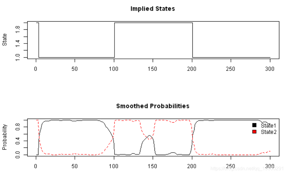
VitPath = viterbi(ResFit, y)DimObs = 1
	matplot(fb$Gamma, type='l', main='Smoothed Probabilities', ylab='Probability')
		legend(x='topright', c('State1','State2'),  fill=1:2, bty='n')
![]()
fm2 = fit(mod, verbose = FALSE)Use logLik to converge at iteration 69: 125.6168
	probs = posterior(fm2)

	layout(1:2)
	plot(probs$state, type='s', main='Implied States', xlab='', ylab='State')

	matplot(probs[,-1], type='l', main='Probabilities', ylab='Probability')
		legend(x='topright', c('State1','State2'),  fill=1:2, bty='n')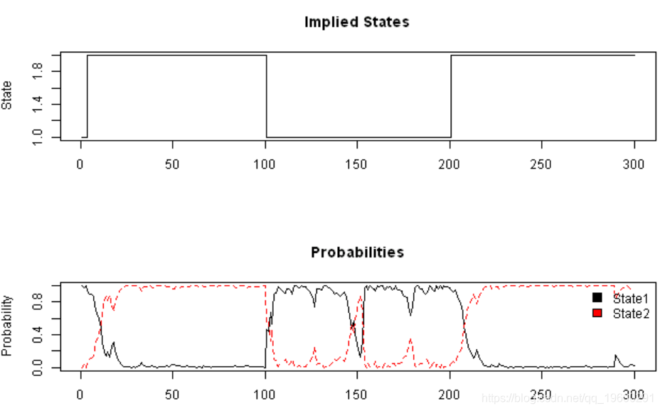
![]()
	#*****************************************************************
	# Add some data and see if the model is able to identify the regimes
	#******************************************************************
	bear2  = rnorm( 100, -0.01, 0.20 )
	bull3 = rnorm( 100, 0.10, 0.10 )
	bear3  = rnorm( 100, -0.01, 0.25 )
	true.states = c(true.states, rep(2,100),rep(1,100),rep(2,100))
	y = c( bull1, bear,  bull2, bear2, bull3, bear3 )
DimObs = 1
	plota(data, type='h', x.highlight=T)
		plota.legend('Returns + Detected Regimes')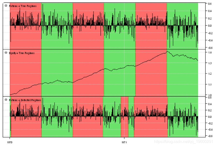
![]()
#*****************************************************************
# Load historical prices
#******************************************************************
data = env()
getSymbols('SPY', src = 'yahoo', from = '1970-01-01', env = data, auto.assign = T)
price = Cl(data$SPY)
open = Op(data$SPY)
ret = diff(log(price))
ret = log(price) - log(open)
atr = ATR(HLC(data$SPY))[,'atr']
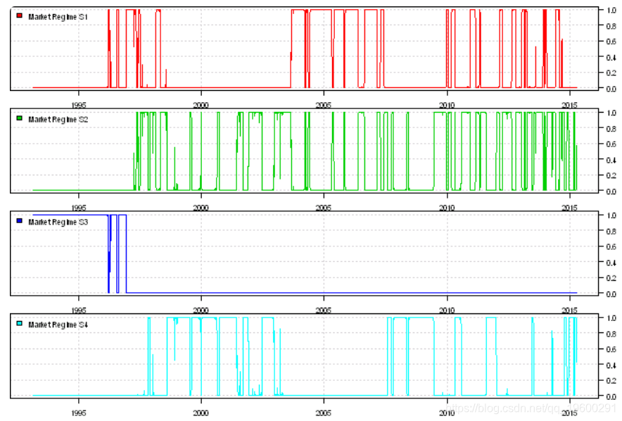
fm2 = fit(mod, verbose = FALSE)Use logLik to converge at iteration 30: 18358.98
print(summary(fm2))
Initial state probabilties model pr1 pr2 pr3 pr4 0 0 1 0

Transition matrix toS1 toS2 toS3 toS4 fromS1 9.821940e-01 1.629595e-02 1.510069e-03 8.514403e-45 fromS2 1.167011e-02 9.790209e-01 8.775478e-68 9.308946e-03 fromS3 3.266616e-03 8.586650e-47 9.967334e-01 1.350529e-69 fromS4 3.608394e-65 1.047516e-02 1.922545e-130 9.895248e-01

Response parameters Resp 1 : gaussian Resp 2 : gaussian Re1.(Intercept) Re1.sd Re2.(Intercept) Re2.sd St1 2.897594e-04 0.006285514 1.1647547 0.1181514 St2 -6.980187e-05 0.008186433 1.6554049 0.1871963 St3 2.134584e-04 0.005694483 0.4537498 0.1564576 St4 -4.459161e-04 0.015419207 2.7558362 0.7297283

 	Re1.(Intercept)	Re1.sd	Re2.(Intercept)	Re2.sd
St1	0.000289759401378951	0.00628551404616354	1.16475474419891	0.118151350440916
St2	-6.98018749098021e-05	0.00818643307634358	1.65540488736983	0.187196307284941
St3	0.000213458358141314	0.00569448330115608	0.453749781945066	0.156457606460757
St4	-0.00044591612667264	0.0154192070819596	2.75583620018895	0.72972830143278
probs = posterior(fm2)

print(head(probs))
rownames(x) state S1 S2 S3 S4
1 3 0 0 1 0
2 3 0 0 1 0
3 3 0 0 1 0
4 3 0 0 1 0
5 3 0 0 1 0
6 3 0 0 1 0
layout(1:3)
plota(temp, type='l', col='darkred')
	plota.legend('Market Regimes', 'darkred')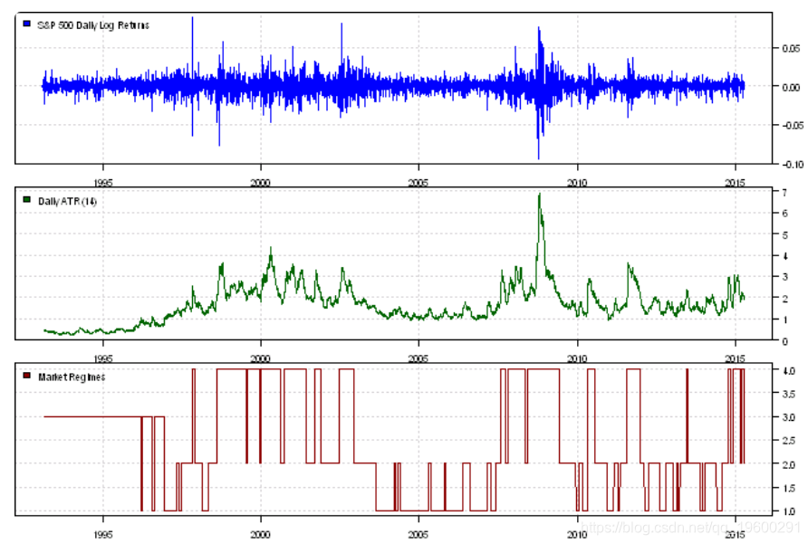
![]()
layout(1:4)
![]()