Improve deep neural networks

Learning materials: deep learning course notes , deeplearning.ai "improving deep neural network", "python deep learning"

Another note, "Structured Machine Learning Project," is helpful for all machine learning projects. This note is specifically aimed at improving neural networks.

1. Solve the problem of overfitting

There are two directions for solving overfitting: reducing the dimension of the parameter space and reducing the effective scale in each dimension . Or you can add data from the source to make the data more comprehensive, but collecting sample data and labeling are often expensive.

Reduce the dimension of the parameter space: reduce model size, reduce parameters, parameter sharing, etc .;

Reduce the effective scale in each dimension : regularization, early stopping, etc.

1. Regularization

There are many different regularization functions, including L1 regularizaion, L2 regularization, dropout regularization, etc. L2 regularization is often used.

L2 regularization

The following figure is: the use of L2 regularization. Used in cost function

L2:

\[\frac{\lambda}{2m}\sum_{i=1}^{n}||W^{[l]}||_2^2 \]

L1:

\[\frac{\lambda}{2m}\sum_{i=1}^{n}||W^{[l]}||_1 \]

\ (\ lambda \) is a regularization parameter and a hyperparameter.

The following is the parameter W to be regularized, referring to: the sum of the squares of all the w parameters

\[||W^{[l]}||_2^2 \]

The meaning of the above figure refers to the gradual reduction of each parameter w

When w is approximately equal to 0, which means that the role of this hidden unit disappears, it means that regularization makes the neural network simple. This is also called "weight loss". During the regularization process, the neural network in Figure 3 is gradually transformed into the simple network in Figure 1, and there will be a good result in the middle.

Dropout regularization

Dropout regularization simplifies the neural network by randomly deactivating some nodes.

Each layer can set the value of keep-prob to make the deactivation rate of each layer different

代码实现：
a_3是指第三层的a的矩阵
keep_prob是概率值   例：keep_prob = 0.8 说明有80%的节点不失活

d_3 = np.random.rand(a_3.shape[0],a_3.shape[1]) < keep_prob
#d_3是一个和a_3相同维度的布尔矩阵

a_3 = np.multipy(a_3,d_3)	#也就是a_3=a_3*d_3
#这个操作决定哪些节点失活了，a_3中乘了false的节点失活

a_3 = a_3/keep_prob			
#inverted dropout反向随机失活的使用，此运算可以很好的计算平均值，避免以后还要计算

2. Add data: data enhancement

Commonly used data augmentation includes mirror image flipping, random cropping, and color conversion. More data samples can be obtained through data enhancement.
Disadvantages: The quality of the newly added data is not high enough, and it is not as good as the new data.
Advantages: The cost is almost 0

3. Early stopping

Only train on the training set, and calculate the error of the model on the verification set every one cycle. When the error of the model on the verification set is worse than the previous training result (or define other stopping rules), stop training, the last time The best case as a training model

Disadvantages: It is impossible to achieve the optimal deviation and variance at the same time.

Advantages: rapid, can effectively avoid overfitting, unlike L2 regularization requires a lot of time to calculate the appropriate value of \ (\ lambda \) hyperparameter.

2. Gradient disappearance, gradient explosion

In a deep neural network, it is possible that the weights of w are all or mostly greater than 1 or less than 1 so that the values ​​passed in the past will continue to increase or decrease exponentially, so that the gradient disappears and the gradient explodes.

Reasonable initialization parameters can effectively alleviate this situation:

WL = np.random.randn(WL.shape[0], WL.shape[1]) * np.sqrt(1/n)

n是输入的神经元个数，即WL.shape[1]

3. Gradient test

When the gradient test is only used for debugging, you can use this method to determine whether there is an error during gradient descent in backpropagation.

For those partial derivatives such as w and b

\ [w = w-dw \]

When using gradient descent, it is sometimes necessary to judge whether dw is correct, and use the gradient test method.

The gradient test is actually solved by the definition of derivative:

\[d\theta=\frac{f(\theta+\omega-f(\theta-\omega))}{2\omega} \]

Calculate whether this result is equal to dw

Practical skills and precautions for gradient testing in neural networks

1. Do not use the gradient test in training, it is only used for debugging. After use, turn off the gradient test function;
2. If the gradient test of the algorithm fails, check all the items and try to find out the bug, that is, determine which dθapprox [i] differs greatly from the value of dθ;
3. When the cost function contains regular terms, you also need to bring regular terms to check;
4. The gradient test cannot be used simultaneously with dropout. Because during each iteration, dropout randomly eliminates different subsets of hidden layer units, it is difficult to calculate the cost function J of dropout on gradient descent. It is recommended to close dropout, double check with gradient test, make sure the algorithm is correct without dropout, and then open dropout;

Four. Optimization algorithm

One of the reasons why deep learning is difficult to maximize its effect in the field of big data is that it is very slow to train on the basis of huge data sets. The optimization algorithm can help to quickly train the model and greatly improve efficiency.

1. BGD

• Batch gradient descent: traverse all data sets to calculate the loss function once, and then calculate the gradient of the function for each parameter and update the gradient. This method needs to read all the samples in the data set every time the parameters are updated. The calculation overhead is large and the calculation speed is slow. Online learning is not supported.

2. SGD

• Stochastic gradient descent (stochastic gradient descent) is to update iteratively through each sample, calculate the loss function for each piece of data, and then find the gradient update.

• Advantages: fast

• Disadvantages: The accuracy is reduced, it may not be globally optimal, and the convergence performance is not very good. It may be dangling around the best advantage, and the two parameter updates may cancel each other out, causing the target function to oscillate more violently.

3. MBGD

In order to overcome the shortcomings of the two methods, a compromise method is generally adopted, mini-batch gradient decent, small batch gradient descent, this method divides the data into several batches, and updates the parameters according to the batch. A set of data in the batch jointly determines the direction of the gradient, and it is not easy to deviate when it descends, reducing the randomness. On the other hand, because the number of samples in a batch is much smaller than the entire data set, the amount of calculation is not very large.

---

• If the size of the training sample is relatively small, such as m ⩽ 2000, choose the batch gradient descent method;
• If the size of the training sample is relatively large, choose the Mini-Batch gradient descent method. In order to adapt to the computer's information storage method, the code runs faster when the mini-batch size is a power of 2. Typical sizes are \ (2 ^ 6 \) , \ (2 ^ 7 \) , \ (2 ^ 8 \) , \ (2 ^ 9 \) . The size of mini-batch should be consistent with CPU / GPU memory.
• The size of the mini-batch is also an important hyperparameter, which needs to be tried quickly based on experience to find the value that can most effectively reduce the cost function.

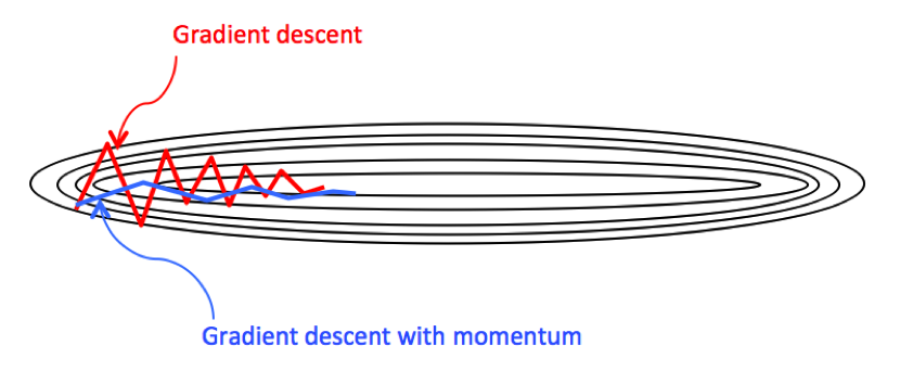
4. Momentum gradient descent method

The momentum gradient descent method is an improvement to MBGD. The main problem of mini-batch is that the function oscillation is larger during training, and the left and right swings are reduced after optimization, thereby improving efficiency.

Exponential weighted average

\ (V_t = \ beta V_ {t-1} + (1- \ beta) \ theta_t \)

The exponential weighted average is the average of the previous \ (\ frac {1} {(1- \ beta)} \) days

Average weighted index and not the most accurate method of calculation of the average, you can calculate directly the last 10 days or 50 days to get a better estimate of the average, but the drawback is the need to take up more memory to save data, perform more complex computing The cost is even higher.

One of the benefits of the exponentially weighted average formula is that it requires only one line of code and takes up very little memory, so it is extremely efficient and saves costs .

Exponential average weighted deviation correction

Momentum gradient descent formula

The idea of ​​the momentum gradient descent method is very simple, that is, the derivative value is first averaged with an exponential average weight , and then the value is used to update the parameter value

5. RMSprop algorithm

RMSProp helps reduce the swing on the path to the minimum value and allows a larger learning rate α to be used to accelerate the algorithm learning speed. Moreover, it and Adam optimization algorithm have been proved to be applicable to different deep learning network structures.

6. Adams algorithm

Adams algorithm is to combine Momentum and RMSProp algorithm together.

The specific process is as follows (l is omitted):

Note: Be sure to correct the deviation

The Adam optimization algorithm has many hyperparameters, among which

• Learning rate α: need to try a series of values ​​to find more suitable;
• β1: The commonly used default value is 0.9;
• β2: The author of Adam algorithm suggested 0.999;
• ϵ: It is not important and will not affect the performance of the algorithm. The author of the Adam algorithm suggests \ (10 ​​^ {-8} \) ;

β1, β2, ϵ usually do not need debugging.

7. Decay in learning rate

For the hyperparameter learning rate \ (\ alpha \) , if a fixed learning rate α is set, near the minimum point, there will be some noise in different batches, so it will not accurately converge, but always at the minimum value Fluctuation around a larger range.

However, if the learning rate α is gradually reduced with time, the initial step size is larger when the initial α is larger, and the gradient can be descended at a faster rate; and the value of α is gradually reduced later, that is, reduced The step size helps the algorithm to converge and it is easier to approach the optimal solution.

8. Local optimal problem

• A saddle point (saddle) is a point where the derivative on the function is zero, but not a local extremum on the axis. When we build a neural network, usually the point where the gradient is zero is the saddle point, not the local minimum.

• When training a large neural network, there are a large number of parameters, and the cost function is defined in a higher dimensional space, it is unlikely to be trapped in such a poor local optimization that all dimensional derivatives are 0 The situation is to reach the saddle point.

• The stationary segment near the saddle point will make learning very slow, which is why the momentum gradient descent method, RMSProp, and Adam optimization algorithms can accelerate learning, and they can help get out of the stationary segment as early as possible.

5. Hyperparameter selection

1. Importance of hyperparameters (not absolute)

2. Assistant skills

Tips for systematically organizing the superparameter debugging process:

• Randomly select points (rather than uniformly select) and use these points to experiment with the effects of hyperparameters. The reason for this is that it is difficult for us to know the importance of hyperparameters in advance, and more experiments can be conducted by selecting more values;
• From coarse to fine: a small area composed of points with good focusing effect, in which values ​​are more densely collected, and so on;

3. Choose the right ruler

• For the learning rate α, it is more reasonable to use a logarithmic scale and the non-linear axis: 0.0001, 0.001, 0.01, 0.1, etc., and then randomly and uniformly take values ​​between these scales;
• For β, taking 0.9 is equivalent to calculating the average value among 10 values, and taking 0.999 is equivalent to calculating the average value among 1000 values. You can consider the value of 1-β, which is similar to the learning rate.

6. Batch Normalization

effect:

1. It will make the parameter search problem easier, make the selection of hyperparameters by the neural network more stable, the range of hyperparameters will be larger, the working effect is very good, and training will be easier.
2. Improve the training speed of the neural network by similarly standardizing the input of each neuron in the hidden layer;
3. It can reduce the impact of the weight change of the front layer on the back layer, and the overall network is more robust.

The previous normalization is to eigenvalues ​​(that is, the input layer), and Batch normalization is used to normalize the value of Z (that is, the hidden layer). Although similar to the normalized eigenvalues, batch norm is not only zero Mean value, unified variance, and the two parameters \ (\ gamma \) and \ (\ beta \) are added, and the mean and variance can be customized. The reason for setting γ and β is that if the input mean of each hidden layer is in a region close to 0, that is, in the linear region of the activation function, it is not conducive to training a nonlinear neural network, resulting in a less effective model. Therefore, we need to use γ and β to further process the normalized results.

When using Batch Normalization, because the normalization process includes a step of subtracting the mean, b does not actually play a role, and its numerical effect is handed over to β. Therefore, in Batch Normalization, b can be omitted or temporarily set to 0. ——So after using Batach Norm, the super parameter becomes \ (W \) $ \ beta $$ \ gamma $

7. Transfer learning

Transfer learning (Tranfer Learning) is to apply a part of the network structure of the trained neural network model to another model, and apply the knowledge and experience learned from a certain task by one neural network to another task to significantly improve Learning task performance. The migration objects are related. For example, the low-level features of cat and dog recognition and radiology diagnosis are similar. They are all about edge detection of image processing, features of lines, etc. This is the common knowledge of the two learning tasks. In transfer learning, the retraining of these layers can be omitted.

If the new data set is very small, you may only need to retrain the weights of the last layer before the output layer, ie \ (W ^ {[L]}, b ^ {[L]} \) , and keep other parameters unchanged ; If there is enough data, you can just keep the network structure and retrain the coefficients of all layers in the neural network. At this time, the initial weights are obtained from the previous model training. This process is called Pre-Training, and the subsequent weight update process is called Fine-Tuning .

It makes sense to carry out transfer learning on the following occasions:

1. Two tasks have the same input (for example, both images or both audio);
2. Tasks with more data are migrated to tasks with less data ;
3. The low-level features of a task (some functions of the underlying neural network) are helpful for learning another task.

Model fine-tuning steps

1. Add a custom network to the already trained base network
2. Freeze network
3. The added part of the training
4. Unfreeze some layers of the base network
5. Joint training to unfreeze these layers and added parts

Model fine-tuning is to unfreeze the previously trained network after training the network defined later. Model fine-tuning generally unfreezes some layers of the top layer because the bottom layer is more versatile.

The data set is very small, and fine-tuning is not necessary; if the data set is large, some layers of fine-tuning can be properly thawed, and all pre-trained networks can be trained as initial values.