CS231n Lecture5-Convolutional Neural Networks Study Notes

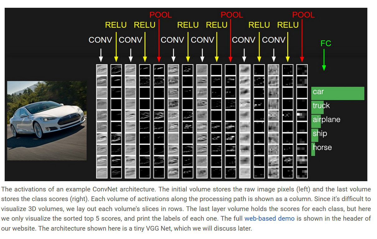
一、Architecture Overview

• Regular Neural Nets and Convolutional Neural Networks(插图)
  

1. Layers used to build ConvNets

• Usually convolution layer, pooled layer, fully connected layers.
• However, the convolution between the layers and the cell layer, generally has an active function layer
• Each layer receives a three-dimensional parameter is input, while the output of a three-dimensional data by different functions
• And a convolution layer fully connected layer parameters; activated cell layer and the function layer has no parameters.
• Convolution layer, fully connected layers and layers pool may have additional hyper-parameters, but no activation function layer.
• Illustration explain
  

二、Convolutional Layer

1. Local Connectivity: We used convolution kernel (or called receptive fields receptive field) connection, this part is the difference between before and ordinary neural network parameters of this section is shared, you can save a lot of resources.

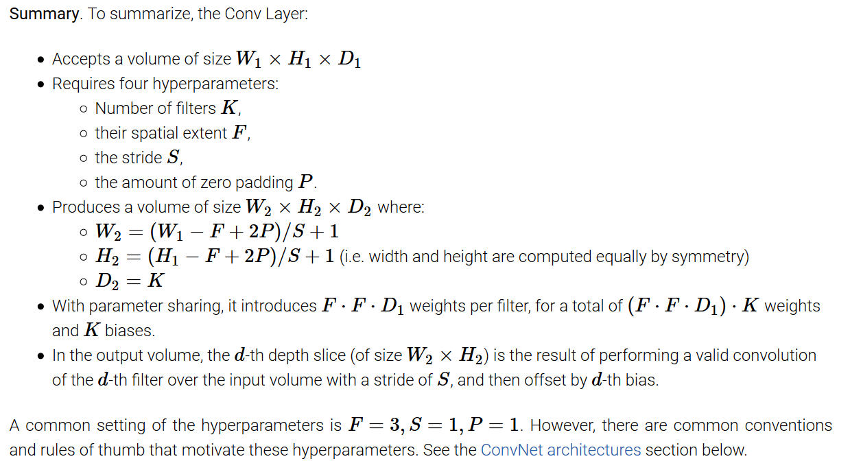
2. Spatial arrangement: three super important parameter, a depth (depth), step (stride), 0 is filled (zero-padding). I.e. the depth of the number of channels in the output, the number of the convolution kernel is much depth; and the convolution step is sliding on the image size; 0 is filled around the input data is filled in on all-0 data.

3. Calculating an output size: size of the input size of W; the size of the convolution kernel F; step size S; size 0 filled P; output size is (W-F+2*P)/S+1(Illustration)
   

4. Filled with 0s reason: that is, holding the same size input and output size of the size; also sometimes setting step, if the filler is not used, the output is the case there will be a decimal, then is invalid, and therefore needs to be filled.

5. Parameter Sharing: is talking about the parameters of the convolution kernel is shared.

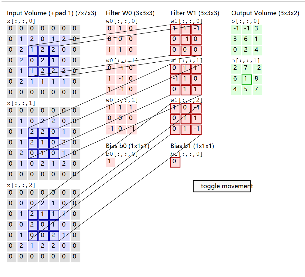
6. Convolution kernel and how the local area operations: We know the general form is a convolution kernel 5x5x3, 3represents the depth of the original input data, i.e., number of channels, we are drawn into to the convolution kernel in a practice a dimensional vector convolution kernel while the overlap portion is also stretched into a 5x5x3=75one-dimensional vector, the two parts can be a dot product operation. Finally, get a number, which is a convolution Nucleation pixel newly generated. For example, into the original size 227x227x3, the size of the convolution kernel 11x11x3=363, step size 4, without using a filler, calculated according to the formula (227-11)/4+1=55, the number of the convolution kernel used is 96one, meaning the number of channels for output size 96, output size becomes 55x55x96, with the foregoing explanation is partially drawn as a convolution kernel dimensional vector, it can be viewed as the convolution kernel 96x363and the input 363x3025matrix multiplication, which is the final result of the dot product96x3025=55x55x96

7. Backpropagation: convolution operation (for weight and weight data) is also transmitted to the convolution (but using flip space filter)

8. 1x1 convolution:

9. Dilated convolutions:

10. Case:
    

三、Pooling Layer, Normalization Layer and Fully-connected layer

• Simple terms is downsampling, to reduce the size, the control overfitting, is retained without changing the depth, i.e. the number of channels.

1. Sizing: Illustration
   

2. General pooling: General pooled maximum, average pooling, L2 paradigm pooled.

3. Backpropagation:

4. Some network structure layer may also be discarded pool

5. Normalization layer , has failed in a number of network structure, while a number of experiments have proved that this part of the contribution to the results is very small.

6. Fully connected layers , the last layer is drawn into a one-dimensional vector data, a subsequent operation, for each type of generated score.

四、Converting FC layers to CONV layers

1. I did not know

五、ConvNet Architectures

1. INPUT -> [[CONV -> RELU]*N -> POOL?]*M -> [FC -> RELU]*K -> FC
2. Usually a convolutional network structure as shown above, N is the number of repetitions is generally greater than the module 0is less than 3, the number of other parameters the same way.
3. I prefer to use several small convolution kernel level rather than a large convolution kernel layer to achieve the size of the same size. The following reasons: 1. The multilayer layer comprises linear convolution, characterized in that they are more expressive; 2. the use of fewer parameters express more powerful input characteristics. Cons: may need more memory to accommodate the results of all intermediate convolution layer, if we reverse the spread.
4. Some common parameters, typically the size of the input 32, 64, 96, 224, 384, 512, the convolution convolution kernel layer Fand the step size Sand the filling Pof the relationship, assuming step size S = 1, if you want to maintain the original size, thenP = (F - 1)/2
5. Why use stride of 1 in CONV? Allow us more space pooled specimens to the layer, while at the same time convert only the number of channels.
6. Why use padding? In addition to maintaining the same space previously mentioned, can also improve performance, more efficient extraction of the feature information, because excessive downsized lost a lot of useful information.

六、Case Studies

1. LeNet: 1990s successfully applied convolution network, is used to identify postal codes. Paper

2. AlexNet: The first popular work on computer vision, in 2012 ImageNet ILSVRC challenge game scores far higher than the second. The structure and LeNet acquaintance, but the network deeper and bigger. Paper

3. ZF Net: it is an improvement AlexNet by adjusting parameters over architecture, particularly by expanding the size of the convolution intermediate layer, and the size of the first filter layer and smaller stride. Paper

4. GoogLeNet: 2014 Nian ILSVRC winners are Szegedy, who convolution network from Google. Its main contribution is to start the development of the module, the module dramatically reduces the number of parameters of the network (4M, and AlexNet only 60M). In addition, as used herein, the average pool at the top of ConvNet rather than layer fully connected, eliminating a lot of it seems less important parameters. Paper

5. VGGNet: 2014 Nian ILSVRC runner-up is Karen Simonyan and Andrew Zisserman founded VGGNet. Its main contribution is to show the depth of the network is a key component of good performance. Their ultimate best network includes 16 CONV / FC layers, and the interest is, has a very homogeneous structure, only to end the execution of the convolution pool 3x3 and 2x2 from the start. They pre-trained models can plug and play in caffe in. One drawback is that it VGGNet greater computational overhead and uses more memory and parameters (140 million). Most of these parameters are located on a fully connected layers, and since then, we find that FC can remove these layers without sacrificing performance, thus significantly reducing the number of required parameters. Paper

6. ResNet: won the 2015 championship by the ILSVRC He Kaiming, who developed residual network. It has a special connector and a large number of skipped using batch standardization. The architecture also lacks a fully connected network layer ends. Readers can also refer to kaim demo (video, slides), and some recent experiments copy of these networks in the Torch. ResNets is currently the most advanced convolution neural network model, the default choice is to use convolution neural networks in practice (May 10, 2016 ended). Of particular note is that recently there have been more changes. Paper

7. VGGNet in detail.:

INPUT: [224x224x3]        memory:  224*224*3=150K   weights: 0
CONV3-64: [224x224x64]  memory:  224*224*64=3.2M   weights: (3*3*3)*64 = 1,728
CONV3-64: [224x224x64]  memory:  224*224*64=3.2M   weights: (3*3*64)*64 = 36,864
POOL2: [112x112x64]  memory:  112*112*64=800K   weights: 0
CONV3-128: [112x112x128]  memory:  112*112*128=1.6M   weights: (3*3*64)*128 = 73,728
CONV3-128: [112x112x128]  memory:  112*112*128=1.6M   weights: (3*3*128)*128 = 147,456
POOL2: [56x56x128]  memory:  56*56*128=400K   weights: 0
CONV3-256: [56x56x256]  memory:  56*56*256=800K   weights: (3*3*128)*256 = 294,912
CONV3-256: [56x56x256]  memory:  56*56*256=800K   weights: (3*3*256)*256 = 589,824
CONV3-256: [56x56x256]  memory:  56*56*256=800K   weights: (3*3*256)*256 = 589,824
POOL2: [28x28x256]  memory:  28*28*256=200K   weights: 0
CONV3-512: [28x28x512]  memory:  28*28*512=400K   weights: (3*3*256)*512 = 1,179,648
CONV3-512: [28x28x512]  memory:  28*28*512=400K   weights: (3*3*512)*512 = 2,359,296
CONV3-512: [28x28x512]  memory:  28*28*512=400K   weights: (3*3*512)*512 = 2,359,296
POOL2: [14x14x512]  memory:  14*14*512=100K   weights: 0
CONV3-512: [14x14x512]  memory:  14*14*512=100K   weights: (3*3*512)*512 = 2,359,296
CONV3-512: [14x14x512]  memory:  14*14*512=100K   weights: (3*3*512)*512 = 2,359,296
CONV3-512: [14x14x512]  memory:  14*14*512=100K   weights: (3*3*512)*512 = 2,359,296
POOL2: [7x7x512]  memory:  7*7*512=25K  weights: 0
FC: [1x1x4096]  memory:  4096  weights: 7*7*512*4096 = 102,760,448
FC: [1x1x4096]  memory:  4096  weights: 4096*4096 = 16,777,216
FC: [1x1x1000]  memory:  1000 weights: 4096*1000 = 4,096,000

TOTAL memory: 24M * 4 bytes ~= 93MB / image (only forward! ~*2 for bwd)
TOTAL params: 138M parameters

七、Computational Considerations

• There are three major sources of memory to keep track of:

1. Storing the intermediate data
2. Size of the parameter, the gradient
3. You must maintain a wide variety of memory, such as image data pieces, maybe they enhanced version, and so on.