文章目录
UR5机械臂正逆运动学
1. DH参数与坐标系
标准DH参数的连杆坐标系建立在传动轴,改进DH参数的连杆坐标系建立在驱动轴,对于UR5这类串联型机械臂,这两种DH参数法没有优劣之分。
1.1 UR5 Standard DH Parameter
(for other model please click here)
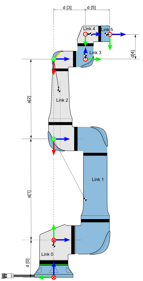
| Kinematics | θ i \theta_i θi [rad] | a i a_i ai [m] | d i d_i di [m] | α i \alpha_i αi [rad] |
|---|---|---|---|---|
| Joint 1 | 0 | 0 | 0.089159 | π/2 |
| Joint 2 | 0 | -0.42500 | 0 | 0 |
| Joint 3 | 0 | -0.39225 | 0 | 0 |
| Joint 4 | 0 | 0 | 0.10915 | π/2 |
| Joint 5 | 0 | 0 | 0.09465 | -π/2 |
| Joint 6 | 0 | 0 | 0.0823 | 0 |

MatLab程序:
% startup_rvc
clear;clc;
%UR5 standard_DH parameter
a=[0,-0.42500,-0.39225,0,0,0];
d=[0.089159,0,0,0.10915,0.09465,0.08230];
alpha=[pi/2,0,0,pi/2,-pi/2,0];

% 建立UR5机械臂模型
L1 = Link('d', d(1),  'a', a(1), 'alpha', alpha(1),  'standard');
L2 = Link('d', d(2),  'a', a(2), 'alpha', alpha(2),  'standard');
L3 = Link('d', d(3),  'a', a(3), 'alpha', alpha(3),  'standard');
L4 = Link('d', d(4),  'a', a(4), 'alpha', alpha(4),  'standard');
L5 = Link('d', d(5),  'a', a(5), 'alpha', alpha(5),  'standard');
L6 = Link('d', d(6),  'a', a(6), 'alpha', alpha(6),  'standard');
tool_robot = SerialLink([L1,L2,L3,L4,L5,L6], 'name', 'UR5');
tool_robot.display();
view(3);
tool_robot.teach();
UR5机械臂模型:

1.2 UR5 Modify DH Parameter

| Kinematics | θ i \theta_i θi [rad] | a i − 1 a_{i-1} ai−1 [m] | d i d_i di [m] | α i − 1 \alpha_{i-1} αi−1 [rad] |
|---|---|---|---|---|
| Joint 1 | 0 | 0 | 0.089159 | 0 |
| Joint 2 | 0 | 0 | 0 | π/2 |
| Joint 3 | 0 | -0.42500 | 0 | 0 |
| Joint 4 | 0 | -0.39225 | 0.10915 | 0 |
| Joint 5 | 0 | 0 | 0.09465 | π/2 |
| Joint 6 | 0 | 0 | 0.08230 | -π/2 |
2. Forward kinematics
正运动学:已知机械臂六个关节角度求变换矩阵T
2.1 正运动学解算(标准DH参数)
i i − 1 T = R o t ( z , θ i ) ⋅ T r a n s ( 0 , 0 , d i ) ⋅ R o t ( x , α i ) ⋅ T r a n s ( a i , 0 , 0 ) _{i}^{i-1}T=Rot(z,\theta_i)\cdot Trans(0,0,d_i) \cdot Rot(x,\alpha_{i})\cdot Trans(a_{i},0,0) ii−1T=Rot(z,θi)⋅Trans(0,0,di)⋅Rot(x,αi)⋅Trans(ai,0,0)
整理得:
i i − 1 T = ( cos ( θ i ) − sin ( θ i ) 0 0 sin ( θ i ) cos ( θ i ) 0 0 0 0 1 0 0 0 0 1 ) ( 1 0 0 0 0 1 0 0 0 0 1 d i 0 0 0 1 ) ( 1 0 0 0 0 cos ( α i ) − sin ( α i ) 0 0 sin ( α i ) cos ( α i ) 0 0 0 0 1 ) ( 1 0 0 a i 0 1 0 0 0 0 1 0 0 0 0 1 ) _{i}^{i-1}T=\begin{pmatrix}\cos(\theta_{i}) & -\sin(\theta_{i}) & 0 & 0\\ \sin(\theta_{i}) & \cos(\theta_{i}) & 0 & 0\\ 0 & 0 & 1 & 0\\ 0 & 0 & 0 & 1\end{pmatrix}\begin{pmatrix}1 & 0 & 0 & 0\\ 0 & 1 & 0 & 0\\ 0 & 0 & 1 & \mathrm{d}_{i}\\ 0 & 0 & 0 & 1\end{pmatrix}\begin{pmatrix}1 & 0 & 0 & 0\\ 0 & \cos(\alpha_{i}) & -\sin(\alpha_{i}) & 0\\ 0 & \sin(\alpha_{i}) & \cos(\alpha_{i}) & 0\\ 0 & 0 & 0 & 1\end{pmatrix}\begin{pmatrix}1 & 0 & 0 & a_{i} & \\ 0 & 1 & 0 & 0 & \\ 0 & 0 & 1 & 0 & \\ 0 & 0 & 0 & 1 & \end{pmatrix} ii−1T=
cos(θi)sin(θi)00−sin(θi)cos(θi)0000100001
10000100001000di1
10000cos(αi)sin(αi)00−sin(αi)cos(αi)00001
100001000010ai001

整理得:
i i − 1 T = [ cos ( θ i ) − sin ( θ i ) cos ( α i ) sin ( θ i ) sin ( α i ) a i cos ( θ i ) sin ( θ i ) cos ( θ i ) cos ( α i ) − cos ( θ i ) sin ( α i ) a i sin ( θ i ) 0 sin ( α i ) cos ( α i ) d i 0 0 0 1 ] _{i}^{i-1}T=\begin{bmatrix}\cos(\theta_i)&-\sin(\theta_i)\cos(\alpha_{i})&\sin(\theta_i)\sin(\alpha_{i})&a_{i}\cos(\theta_i)\\\sin(\theta_i)&\cos(\theta_i)\cos(\alpha_{i})&-\cos(\theta_i)\sin(\alpha_{i})&a_{i}\sin(\theta_i)\\0&\sin(\alpha_{i})&\cos(\alpha_{i})&d_i\\0&0&0&1\end{bmatrix} ii−1T=
cos(θi)sin(θi)00−sin(θi)cos(αi)cos(θi)cos(αi)sin(αi)0sin(θi)sin(αi)−cos(θi)sin(αi)cos(αi)0aicos(θi)aisin(θi)di1
机械臂末端坐标系 6 相对笛卡尔基坐标系 0 的齐次变换矩阵 6 0 T _{6}^{0}T 60T:
6 0 T = 1 0 T ⋅ 2 1 T ⋅ 3 2 T ⋅ 4 3 T ⋅ 5 4 T ⋅ 6 5 T _{6}^{0}T = _{1}^{0}T \cdot _{2}^{1}T \cdot _{3}^{2}T \cdot_{4}^{3}T \cdot_{5}^{4}T \cdot _{6}^{5}T 60T=10T⋅21T⋅32T⋅43T⋅54T⋅65T
整理得正运动学方程:
6 0 T = [ n x o x a x p x n y o y a y p y n z o z a z p z 0 0 0 1 ] _{6}^{0}T =\begin{bmatrix} n_x & o_x & a_x & p_x \\n_y & o_y & a_y & p_y\\n_z & o_z & a_z & p_z\\0 & 0 & 0 & 1 \end{bmatrix} 60T=
nxnynz0oxoyoz0axayaz0pxpypz1
{ n x = cos ( θ 6 ) ( sin ( θ 1 ) sin ( θ 5 ) + cos ( θ 2 + θ 3 + θ 4 ) cos ( θ 1 ) cos ( θ 5 ) ) − sin ( θ 2 + θ 3 + θ 4 ) cos ( θ 1 ) sin ( θ 6 ) n y = − cos ( θ 6 ) ( cos ( θ 1 ) sin ( θ 5 ) − cos ( θ 2 + θ 3 + θ 4 ) cos ( θ 5 ) sin ( θ 1 ) ) − sin ( θ 2 + θ 3 + θ 4 ) sin ( θ 1 ) sin ( θ 6 ) n z = cos ( θ 2 + θ 3 + θ 4 ) sin ( θ 6 ) + sin ( θ 2 + θ 3 + θ 4 ) cos ( θ 5 ) cos ( θ 6 ) \begin{cases} n_x = \cos\left(\theta _{6}\right)\,\left(\sin\left(\theta _{1}\right)\,\sin\left(\theta _{5}\right)+\cos\left(\theta _{2}+\theta _{3}+\theta _{4}\right)\,\cos\left(\theta _{1}\right)\,\cos\left(\theta _{5}\right)\right)-\sin\left(\theta _{2}+\theta _{3}+\theta _{4}\right)\,\cos\left(\theta _{1}\right)\,\sin\left(\theta _{6}\right) \\ n_y = -\cos\left(\theta _{6}\right)\,\left(\cos\left(\theta _{1}\right)\,\sin\left(\theta _{5}\right)-\cos\left(\theta _{2}+\theta _{3}+\theta _{4}\right)\,\cos\left(\theta _{5}\right)\,\sin\left(\theta _{1}\right)\right)-\sin\left(\theta _{2}+\theta _{3}+\theta _{4}\right)\,\sin\left(\theta _{1}\right)\,\sin\left(\theta _{6}\right) \\ n_z = \cos\left(\theta _{2}+\theta _{3}+\theta _{4}\right)\,\sin\left(\theta _{6}\right)+\sin\left(\theta _{2}+\theta _{3}+\theta _{4}\right)\,\cos\left(\theta _{5}\right)\,\cos\left(\theta _{6}\right) \end{cases} ⎩ ⎨ ⎧nx=cos(θ6)(sin(θ1)sin(θ5)+cos(θ2+θ3+θ4)cos(θ1)cos(θ5))−sin(θ2+θ3+θ4)cos(θ1)sin(θ6)ny=−cos(θ6)(cos(θ1)sin(θ5)−cos(θ2+θ3+θ4)cos(θ5)sin(θ1))−sin(θ2+θ3+θ4)sin(θ1)sin(θ6)nz=cos(θ2+θ3+θ4)sin(θ6)+sin(θ2+θ3+θ4)cos(θ5)cos(θ6)
{ o x = − sin ( θ 6 ) ( sin ( θ 1 ) sin ( θ 5 ) + cos ( θ 2 + θ 3 + θ 4 ) cos ( θ 1 ) cos ( θ 5 ) ) − sin ( θ 2 + θ 3 + θ 4 ) cos ( θ 1 ) cos ( θ 6 ) o y = sin ( θ 6 ) ( cos ( θ 1 ) sin ( θ 5 ) − cos ( θ 2 + θ 3 + θ 4 ) cos ( θ 5 ) sin ( θ 1 ) ) − sin ( θ 2 + θ 3 + θ 4 ) cos ( θ 6 ) sin ( θ 1 ) o z = cos ( θ 2 + θ 3 + θ 4 ) cos ( θ 6 ) − sin ( θ 2 + θ 3 + θ 4 ) cos ( θ 5 ) sin ( θ 6 ) \begin{cases} o_x = -\sin\left(\theta _{6}\right)\,\left(\sin\left(\theta _{1}\right)\,\sin\left(\theta _{5}\right)+\cos\left(\theta _{2}+\theta _{3}+\theta _{4}\right)\,\cos\left(\theta _{1}\right)\,\cos\left(\theta _{5}\right)\right)-\sin\left(\theta _{2}+\theta _{3}+\theta _{4}\right)\,\cos\left(\theta _{1}\right)\,\cos\left(\theta _{6}\right) \\ o_y = \sin\left(\theta _{6}\right)\,\left(\cos\left(\theta _{1}\right)\,\sin\left(\theta _{5}\right)-\cos\left(\theta _{2}+\theta _{3}+\theta _{4}\right)\,\cos\left(\theta _{5}\right)\,\sin\left(\theta _{1}\right)\right)-\sin\left(\theta _{2}+\theta _{3}+\theta _{4}\right)\,\cos\left(\theta _{6}\right)\,\sin\left(\theta _{1}\right) \\ o_z = \cos\left(\theta _{2}+\theta _{3}+\theta _{4}\right)\,\cos\left(\theta _{6}\right)-\sin\left(\theta _{2}+\theta _{3}+\theta _{4}\right)\,\cos\left(\theta _{5}\right)\,\sin\left(\theta _{6}\right) \end{cases} ⎩ ⎨ ⎧ox=−sin(θ6)(sin(θ1)sin(θ5)+cos(θ2+θ3+θ4)cos(θ1)cos(θ5))−sin(θ2+θ3+θ4)cos(θ1)cos(θ6)oy=sin(θ6)(cos(θ1)sin(θ5)−cos(θ2+θ3+θ4)cos(θ5)sin(θ1))−sin(θ2+θ3+θ4)cos(θ6)sin(θ1)oz=cos(θ2+θ3+θ4)cos(θ6)−sin(θ2+θ3+θ4)cos(θ5)sin(θ6)
{ a x = cos ( θ 5 ) sin ( θ 1 ) − cos ( θ 2 + θ 3 + θ 4 ) cos ( θ 1 ) sin ( θ 5 ) a y = − cos ( θ 1 ) cos ( θ 5 ) − cos ( θ 2 + θ 3 + θ 4 ) sin ( θ 1 ) sin ( θ 5 ) a z = − sin ( θ 2 + θ 3 + θ 4 ) sin ( θ 5 ) \begin{cases} a_x = \cos\left(\theta _{5}\right)\,\sin\left(\theta _{1}\right)-\cos\left(\theta _{2}+\theta _{3}+\theta _{4}\right)\,\cos\left(\theta _{1}\right)\,\sin\left(\theta _{5}\right) \\ a_y = -\cos\left(\theta _{1}\right)\,\cos\left(\theta _{5}\right)-\cos\left(\theta _{2}+\theta _{3}+\theta _{4}\right)\,\sin\left(\theta _{1}\right)\,\sin\left(\theta _{5}\right) \\ a_z = -\sin\left(\theta _{2}+\theta _{3}+\theta _{4}\right)\,\sin\left(\theta _{5}\right) \end{cases} ⎩ ⎨ ⎧ax=cos(θ5)sin(θ1)−cos(θ2+θ3+θ4)cos(θ1)sin(θ5)ay=−cos(θ1)cos(θ5)−cos(θ2+θ3+θ4)sin(θ1)sin(θ5)az=−sin(θ2+θ3+θ4)sin(θ5)
{ p x = d 6 ( cos ( θ 5 ) sin ( θ 1 ) − cos ( θ 2 + θ 3 + θ 4 ) cos ( θ 1 ) sin ( θ 5 ) ) + d 4 sin ( θ 1 ) + a 2 cos ( θ 1 ) cos ( θ 2 ) + d 5 sin ( θ 2 + θ 3 + θ 4 ) cos ( θ 1 ) + a 3 cos ( θ 1 ) cos ( θ 2 ) cos ( θ 3 ) − a 3 cos ( θ 1 ) sin ( θ 2 ) sin ( θ 3 ) p y = a 2 cos ( θ 2 ) sin ( θ 1 ) − d 4 cos ( θ 1 ) − d 6 ( cos ( θ 1 ) cos ( θ 5 ) + cos ( θ 2 + θ 3 + θ 4 ) sin ( θ 1 ) sin ( θ 5 ) ) + d 5 sin ( θ 2 + θ 3 + θ 4 ) sin ( θ 1 ) + a 3 cos ( θ 2 ) cos ( θ 3 ) sin ( θ 1 ) − a 3 sin ( θ 1 ) sin ( θ 2 ) sin ( θ 3 ) p z = d 1 + d 5 ( sin ( θ 2 + θ 3 ) sin ( θ 4 ) − cos ( θ 2 + θ 3 ) cos ( θ 4 ) ) + a 3 sin ( θ 2 + θ 3 ) + a 2 sin ( θ 2 ) − d 6 sin ( θ 5 ) ( cos ( θ 2 + θ 3 ) sin ( θ 4 ) + sin ( θ 2 + θ 3 ) cos ( θ 4 ) ) \begin{cases} p_x = d_{6}\,\left(\cos\left(\theta _{5}\right)\,\sin\left(\theta _{1}\right)-\cos\left(\theta _{2}+\theta _{3}+\theta _{4}\right)\,\cos\left(\theta _{1}\right)\,\sin\left(\theta _{5}\right)\right)+d_{4}\,\sin\left(\theta _{1}\right)+a_{2}\,\cos\left(\theta _{1}\right)\,\cos\left(\theta _{2}\right)+d_{5}\,\sin\left(\theta _{2}+\theta _{3}+\theta _{4}\right)\,\cos\left(\theta _{1}\right)+a_{3}\,\cos\left(\theta _{1}\right)\,\cos\left(\theta _{2}\right)\,\cos\left(\theta _{3}\right)-a_{3}\,\cos\left(\theta _{1}\right)\,\sin\left(\theta _{2}\right)\,\sin\left(\theta _{3}\right) \\ p_y = a_{2}\,\cos\left(\theta _{2}\right)\,\sin\left(\theta _{1}\right)-d_{4}\,\cos\left(\theta _{1}\right)-d_{6}\,\left(\cos\left(\theta _{1}\right)\,\cos\left(\theta _{5}\right)+\cos\left(\theta _{2}+\theta _{3}+\theta _{4}\right)\,\sin\left(\theta _{1}\right)\,\sin\left(\theta _{5}\right)\right)+d_{5}\,\sin\left(\theta _{2}+\theta _{3}+\theta _{4}\right)\,\sin\left(\theta _{1}\right)+a_{3}\,\cos\left(\theta _{2}\right)\,\cos\left(\theta _{3}\right)\,\sin\left(\theta _{1}\right)-a_{3}\,\sin\left(\theta _{1}\right)\,\sin\left(\theta _{2}\right)\,\sin\left(\theta _{3}\right) \\ p_z = d_{1}+d_{5}\,\left(\sin\left(\theta _{2}+\theta _{3}\right)\,\sin\left(\theta _{4}\right)-\cos\left(\theta _{2}+\theta _{3}\right)\,\cos\left(\theta _{4}\right)\right)+a_{3}\,\sin\left(\theta _{2}+\theta _{3}\right)+a_{2}\,\sin\left(\theta _{2}\right)-d_{6}\,\sin\left(\theta _{5}\right)\,\left(\cos\left(\theta _{2}+\theta _{3}\right)\,\sin\left(\theta _{4}\right)+\sin\left(\theta _{2}+\theta _{3}\right)\,\cos\left(\theta _{4}\right)\right) \end{cases} ⎩ ⎨ ⎧px=d6(cos(θ5)sin(θ1)−cos(θ2+θ3+θ4)cos(θ1)sin(θ5))+d4sin(θ1)+a2cos(θ1)cos(θ2)+d5sin(θ2+θ3+θ4)cos(θ1)+a3cos(θ1)cos(θ2)cos(θ3)−a3cos(θ1)sin(θ2)sin(θ3)py=a2cos(θ2)sin(θ1)−d4cos(θ1)−d6(cos(θ1)cos(θ5)+cos(θ2+θ3+θ4)sin(θ1)sin(θ5))+d5sin(θ2+θ3+θ4)sin(θ1)+a3cos(θ2)cos(θ3)sin(θ1)−a3sin(θ1)sin(θ2)sin(θ3)pz=d1+d5(sin(θ2+θ3)sin(θ4)−cos(θ2+θ3)cos(θ4))+a3sin(θ2+θ3)+a2sin(θ2)−d6sin(θ5)(cos(θ2+θ3)sin(θ4)+sin(θ2+θ3)cos(θ4))
6 0 T _{6}^{0}T 60T计算程序:
syms theta1 theta2 theta3 theta4 theta5 theta6 d1 d4 d5 d6 a2 a3
t01 = [cos(theta1), 0, sin(theta1), 0;
       sin(theta1), 0, -cos(theta1), 0;
       0, 1, 0, d1;
       0, 0, 0, 1];

t12 = [cos(theta2), -sin(theta2), 0, a2 * cos(theta2);
       sin(theta2), cos(theta2), 0, a2 * sin(theta2);
       0, 0, 1, 0;
       0, 0, 0, 1];

t23 = [cos(theta3), -sin(theta3), 0, a3 * cos(theta3);
       sin(theta3), cos(theta3), 0, a3 * sin(theta3);
       0, 0, 1, 0;
       0, 0, 0, 1];

t34 = [cos(theta4), 0, sin(theta4), 0;
       sin(theta4), 0, -cos(theta4), 0;
       0, 1, 0, d4;
       0, 0, 0, 1];

t45 = [cos(theta5), 0, -sin(theta5), 0;
       sin(theta5), 0, cos(theta5), 0;
       0, -1, 0, d5;
       0, 0, 0, 1];

t56 = [cos(theta6), -sin(theta6), 0, 0;
       sin(theta6), cos(theta6), 0, 0;
       0, 0, 1, d6;
       0, 0, 0, 1];

T = simplify(t01 * t12 * t23 * t34 * t45 * t56);

% 转换为 LaTeX 格式
latex_T = latex(T);

% 输出结果
disp(latex_T);
2.2 MatLab仿真验证
2.2.1 Matlab程序
function T = forward_kinematics(theta,d,a,alpha)
%forward kenematics
%input:theta(rad)
%output:T

% UR5 standard_DH parameter
% a=[0,-0.42500,-0.39225,0,0,0];
% d=[0.089159,0,0,0.10915,0.09465,0.08230];
% alpha=[pi/2,0,0,pi/2,-pi/2,0];

T01=T_para(theta(1),d(1),a(1),alpha(1));
T12=T_para(theta(2),d(2),a(2),alpha(2));
T23=T_para(theta(3),d(3),a(3),alpha(3));
T34=T_para(theta(4),d(4),a(4),alpha(4));
T45=T_para(theta(5),d(5),a(5),alpha(5));
T56=T_para(theta(6),d(6),a(6),alpha(6));

T=T01*T12*T23*T34*T45*T56;
% T = [nx ox ax px
%      ny oy ay py
%      nz oz az pz
%      0  0  0  1 ]

end
2.2.2 位姿验证
UR仿真器

程序输入:[ 93.14 , -62.68 ,108.27 , -135.56 , -66.46 , 15.59 ]
程序输出:
T = [ − 0.8965 0.1933 0.3988 0.1727 0.2202 0.9752 0.0224 − 0.5555 − 0.3846 0.1078 − 0.9168 0.1110 0 0 0 1 ] T =\begin{bmatrix} \color{blue}-0.8965 & \color{blue}0.1933 & \color{blue}0.3988 & \color{red}{0.1727}\\\color{blue}0.2202& \color{blue}0.9752 & \color{blue}0.0224 & \color{red}{-0.5555}\\\color{blue}-0.3846 & \color{blue}0.1078 & \color{blue}-0.9168 & \color{red}{0.1110}\\0 &0 & 0 & 1 \end{bmatrix} T=
−0.89650.2202−0.384600.19330.97520.107800.39880.0224−0.916800.1727−0.55550.11101
Matlab输出模型:

位置验证:
期望位置(mm): [ 172.69 , -555.55 , 111.06 ]
解算位置(m): p x = 0.1727 p_x = 0.1727 px=0.1727 ; p y = 0.5555 p_y = 0.5555 py=0.5555 ; p z = 0.1110 p_z = 0.1110 pz=0.1110
姿态验证:
期望姿态(rad): 轴角[ 0.297 , 2.719 , 0.093 ]
结算姿态(rad): 旋转矩阵( n x y z n_{xyz} nxyz o x y z o_{xyz} oxyz a x y z a_{xyz} axyz )—>轴角[ 0.2967251, 2.7186044, 0.0934307 ]
[ n x y z o x y z a x y z ] = [ − 0.8965 0.1933 0.3988 0.2202 0.9752 0.0224 − 0.3846 0.1078 − 0.9168 ] ⟺ [ 0.2967251 2.7186044 0.0934307 ] \begin{bmatrix} n_{xyz}&o_{xyz}&a_{xyz} \end{bmatrix} = \begin{bmatrix} -0.8965 &0.1933 &0.3988\\0.2202&0.9752&0.0224\\-0.3846&0.1078&-0.9168 \end{bmatrix} \iff \begin{bmatrix} 0.2967251 &2.7186044 & 0.0934307 \end{bmatrix} [nxyzoxyzaxyz]= −0.89650.2202−0.38460.19330.97520.10780.39880.0224−0.9168 ⟺[0.29672512.71860440.0934307]
3. Inverse kinematics
3.1 逆运动学计算(标准DH参数)
逆运动学是已知变换矩阵 6 0 T _{6}^{0}T 60T(机械臂末端位置和姿态),求六个关节角度。
3.1.1 求解过程
3.1.2 求解公式
- θ 1 \theta_1 θ1(双解)
θ 1 = A tan 2 ( m , n ) − A tan 2 ( d 4 , ± m 2 + n 2 − d 4 2 ) ( 其中 m 2 + n 2 − d 4 2 ≥ 0 ) m = d 6 a y − p y n = a x d 6 − p x \theta_{1}=A\tan2(m,n)-A\tan2(\mathrm{d}_{4},\pm\sqrt{m^{2}+n^{2}-d_{4}^{2}})\qquad(其中m^2+n^2-d_{4}^{2}\geq0)\\ m = d_6a_y-p_y\\ n = a_xd_6-p_x θ1=Atan2(m,n)−Atan2(d4,±m2+n2−d42)(其中m2+n2−d42≥0)m=d6ay−pyn=axd6−px
- θ 5 \theta_5 θ5(双解)
θ 5 = ± arccos ( a x s 1 − a y c 1 ) ( 其中 a x s 1 − a y c 1 ≤ 1 ) \theta_5=\pm\arccos(a_xs_1-a_yc_1)\qquad(其中a_xs_1-a_yc_1\leq1) θ5=±arccos(axs1−ayc1)(其中axs1−ayc1≤1)
- θ 6 \theta_6 θ6
θ 6 = A tan 2 ( m , n ) − A tan 2 ( s 5 , 0 ) ( 其中 s 5 ≠ 0 ) m = n x s 1 − n y c 1 n = o x s 1 − o y c 1 \theta_6=A\tan2(m,n)-A\tan2(s_5,0)\qquad(其中s_5\neq0)\\ m = n_xs_1-n_yc_1\\ n = o_xs_1-o_yc_1 θ6=Atan2(m,n)−Atan2(s5,0)(其中s5=0)m=nxs1−nyc1n=oxs1−oyc1
- θ 3 \theta_3 θ3(双解)
θ 3 = ± arccos ( m 2 + n 2 − a 2 2 − a 3 2 2 a 2 a 3 ) ( 其中 m 2 + n 2 ≤ ( a 2 + a 3 ) 2 ) m = d 5 ( s 6 ( n x c 1 + n y s 1 ) + c 6 ( o x c 1 + o y s 1 ) ) − d 6 ( a x c 1 + a y s 1 ) + p x c 1 + p y s 1 n = p z − d 1 − a z d 6 + d 5 ( o z c 6 + n z s 6 ) \begin{aligned} &\theta_3=\pm\arccos(\frac{m^2+n^2-{a_2}^2-{a_3}^2}{2a_2a_3})\qquad(其中m^2+n^2\leq(a_2+a_3)^2)\\ &m= d_{5}(s_{6}(n_{x}c_{1}+n_{y}s_{1})+c_{6}(o_{x}c_{1}+o_{y}s_{1}))-d_6(a_xc_1+a_ys_1)+p_xc_1+p_ys_1\\ &n=p_{z}-d_{1}-a_{z}d_{6}+d_{5}(o_{z}c_{6}+n_{z}s_{6}) \end{aligned} θ3=±arccos(2a2a3m2+n2−a22−a32)(其中m2+n2≤(a2+a3)2)m=d5(s6(nxc1+nys1)+c6(oxc1+oys1))−d6(axc1+ays1)+pxc1+pys1n=pz−d1−azd6+d5(ozc6+nzs6)
- θ 2 \theta_2 θ2
θ 2 = A tan 2 ( s 2 , c 2 ) s 2 = ( a 3 c 3 + a 2 ) n − a 3 s 3 m a 2 2 + a 3 2 + 2 a 2 a 3 c 3 c 2 = m + a 3 s 3 s 2 a 3 c 3 + a 2 \begin{aligned} &\theta_{2}=A\tan2(s_{2},c_{2})\\ &s_2=\frac{(a_3c_3+a_2)n-a_3s_3m}{a_2^2+a_3^2+2a_2a_3c_3}\\ &c_2=\frac{m+a_3s_3s_2}{a_3c_3+a_2} \end{aligned} θ2=Atan2(s2,c2)s2=a22+a32+2a2a3c3(a3c3+a2)n−a3s3mc2=a3c3+a2m+a3s3s2
- θ 4 \theta_4 θ4
θ 4 = A tan 2 ( − s 6 ( n x c 1 + n y s 1 ) − c 6 ( o x c 1 + o y s 1 ) , o z c 6 + n z s 6 ) − θ 2 − θ 3 \theta_4=A\tan2(-s_6(n_xc_1+n_ys_1)-c_6(o_xc_1+o_y s_1)\;,\;o_zc_6+n_zs_6)-\theta_2-\theta_3 θ4=Atan2(−s6(nxc1+nys1)−c6(oxc1+oys1),ozc6+nzs6)−θ2−θ3
| 算法求解到关节角: | joint 1 | joint 5 | joint 6 | joint 3 | joint 2 | joint 4 |
|---|---|---|---|---|---|---|
| 当前关节角产生解的个数 | 2 | 2 | 1 | 2 | 1 | 1 |
| 当前已有解的个数 | 2 | 4 | 4 | 8 | 8 | 8 |
3.1.3 机械臂奇异点
机械臂的奇异点(Singularity)是指在特定位置或姿态下,机械臂的运动能力受到限制或丧失的情况。在这些点上,机械臂的某些自由度变得不再独立,导致机器人无法在某些方向上移动或控制其末端执行器。
- 奇异点的具体表现:
- 不可逆的运动丧失:在奇异点处,机械臂的某些自由度会出现退化,例如可能无法沿某个方向进行平移或旋转。
- 控制力丧失:如果机械臂的控制系统处于奇异点附近,它可能无法精确地控制末端执行器的位置或姿态。
- 动力学问题:在奇异点时,机械臂的关节力矩可能会变得极大或极小,导致系统不稳定或出现控制问题。
- 常见的奇异点类型:
- 逆向运动学奇异点:在某些位置或姿态下,解算机械臂的逆向运动学方程时可能没有解,或者解的数量不唯一。这种情况通常出现在机械臂的结构或操作空间的特殊配置下。
- Jacobian矩阵的奇异性:Jacobian矩阵描述了机械臂关节速度与末端执行器速度之间的关系。如果Jacobian矩阵在某个点不可逆,表示该点为奇异点。此时,关节速度的控制可能无法完全传递到末端执行器的速度上。
- 如何避免或处理奇异点:
- 路径规划时避开奇异点:通过优化路径或选择合适的轨迹,避免机械臂在操作中经过奇异点。
- 使用冗余自由度:某些机械臂采用冗余自由度(例如额外的自由度或关节),使得在遇到奇异点时,机器人仍然能够继续运动,避免完全的运动丧失。
- 实时控制调整:通过实时监控和动态调整控制算法,使机械臂能够在接近奇异点时适当调整路径。
3.1.4 UR5奇异位置
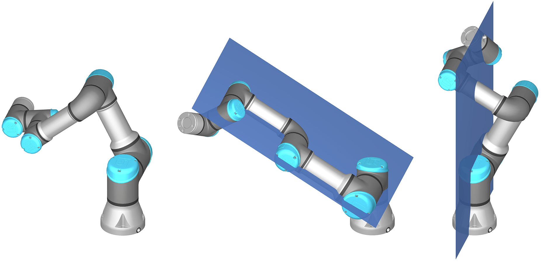
- 腕部奇异(Wrist Singularity)
s 5 = 0 s_5=0 s5=0
θ 5 = 0 \theta_5=0 θ5=0,此时轴线 Z 4 Z_4 Z4和 Z 6 Z_6 Z6平行,逆运动学有无数解
- 肘部奇异(Elbow Singularity)
m 2 + n 2 − ( a 2 + a 3 ) 2 = 0 m = d 5 ( s 6 ( n x c 1 + n y s 1 ) + c 6 ( o x c 1 + o y s 1 ) ) − d 6 ( a x c 1 + a y s 1 ) + p x c 1 + p y s 1 n = p z − d 1 − a z d 6 + d 5 ( o z c 6 + n z s 6 ) m^2+n^2-(a_2+a_3)^2=0\\ \begin{aligned} &m= d_{5}(s_{6}(n_{x}c_{1}+n_{y}s_{1})+c_{6}(o_{x}c_{1}+o_{y}s_{1}))-d_6(a_xc_1+a_ys_1)+p_xc_1+p_ys_1\\ &n=p_{z}-d_{1}-a_{z}d_{6}+d_{5}(o_{z}c_{6}+n_{z}s_{6}) \end{aligned} m2+n2−(a2+a3)2=0m=d5(s6(nxc1+nys1)+c6(oxc1+oys1))−d6(axc1+ays1)+pxc1+pys1n=pz−d1−azd6+d5(ozc6+nzs6)
关节234轴线共面,
- 肩部奇异(Shoulder Singularity)
m 2 + n 2 − d 4 2 = 0 m = d 6 a y − p y n = a x d 6 − p x m^2+n^2-d_{4}^{2}=0\\ m = d_6a_y-p_y\\ n = a_xd_6-p_x m2+n2−d42=0m=d6ay−pyn=axd6−px
关节56交点在 Z 1 Z_1 Z1 Z 2 Z_2 Z2平面内时,发生肩部奇异
3.2 Matlab仿真验证
3.2.1 Matlab程序
function theta = inverse_kinematics(T)

%变换矩阵T已知
%SDH:标准DH参数表求逆解(解析解)
%部分DH参数表如下,需要求解theta信息

%UR5 standard_DH parameter
a=[0,-0.42500,-0.39225,0,0,0];
d=[0.089159,0,0,0.10915,0.09465,0.08230];
alpha=[pi/2,0,0,pi/2,-pi/2,0];% alpha没有用到,故此逆解程序只适合alpha=[pi/2,0,0,pi/2,-pi/2,0]的情况!

nx=T(1,1);ny=T(2,1);nz=T(3,1);
ox=T(1,2);oy=T(2,2);oz=T(3,2);
ax=T(1,3);ay=T(2,3);az=T(3,3);
px=T(1,4);py=T(2,4);pz=T(3,4);

%求解关节角1
m=d(6)*ay-py;  n=ax*d(6)-px;
theta1(1,1)=atan2(m,n)-atan2(d(4),sqrt(m^2+n^2-(d(4))^2));
theta1(1,2)=atan2(m,n)-atan2(d(4),-sqrt(m^2+n^2-(d(4))^2));

%求解关节角5
theta5(1,1:2)=acos(ax*sin(theta1)-ay*cos(theta1));
theta5(2,1:2)=-acos(ax*sin(theta1)-ay*cos(theta1));

%求解关节角6
mm=nx*sin(theta1)-ny*cos(theta1); nn=ox*sin(theta1)-oy*cos(theta1);
%theta6=atan2(mm,nn)-atan2(sin(theta5),0);
theta6(1,1:2)=atan2(mm,nn)-atan2(sin(theta5(1,1:2)),0);
theta6(2,1:2)=atan2(mm,nn)-atan2(sin(theta5(2,1:2)),0);

%求解关节角3
mmm(1,1:2)=d(5)*(sin(theta6(1,1:2)).*(nx*cos(theta1)+ny*sin(theta1))+cos(theta6(1,1:2)).*(ox*cos(theta1)+oy*sin(theta1))) ...
    -d(6)*(ax*cos(theta1)+ay*sin(theta1))+px*cos(theta1)+py*sin(theta1);
nnn(1,1:2)=pz-d(1)-az*d(6)+d(5)*(oz*cos(theta6(1,1:2))+nz*sin(theta6(1,1:2)));
mmm(2,1:2)=d(5)*(sin(theta6(2,1:2)).*(nx*cos(theta1)+ny*sin(theta1))+cos(theta6(2,1:2)).*(ox*cos(theta1)+oy*sin(theta1))) ...
    -d(6)*(ax*cos(theta1)+ay*sin(theta1))+px*cos(theta1)+py*sin(theta1);
nnn(2,1:2)=pz-d(1)-az*d(6)+d(5)*(oz*cos(theta6(2,1:2))+nz*sin(theta6(2,1:2)));
theta3(1:2,:)=acos((mmm.^2+nnn.^2-(a(2))^2-(a(3))^2)/(2*a(2)*a(3)));
theta3(3:4,:)=-acos((mmm.^2+nnn.^2-(a(2))^2-(a(3))^2)/(2*a(2)*a(3)));

%求解关节角2
mmm_s2(1:2,:)=mmm;
mmm_s2(3:4,:)=mmm;
nnn_s2(1:2,:)=nnn;
nnn_s2(3:4,:)=nnn;
s2=((a(3)*cos(theta3)+a(2)).*nnn_s2-a(3)*sin(theta3).*mmm_s2)./ ...
    ((a(2))^2+(a(3))^2+2*a(2)*a(3)*cos(theta3));
c2=(mmm_s2+a(3)*sin(theta3).*s2)./(a(3)*cos(theta3)+a(2));
theta2=atan2(s2,c2);

%整理关节角1 5 6 3 2
theta(1:4,1)=theta1(1,1);theta(5:8,1)=theta1(1,2);
theta(:,2)=[theta2(1,1),theta2(3,1),theta2(2,1),theta2(4,1),theta2(1,2),theta2(3,2),theta2(2,2),theta2(4,2)]';
theta(:,3)=[theta3(1,1),theta3(3,1),theta3(2,1),theta3(4,1),theta3(1,2),theta3(3,2),theta3(2,2),theta3(4,2)]';
theta(1:2,5)=theta5(1,1);theta(3:4,5)=theta5(2,1);
theta(5:6,5)=theta5(1,2);theta(7:8,5)=theta5(2,2);
theta(1:2,6)=theta6(1,1);theta(3:4,6)=theta6(2,1);
theta(5:6,6)=theta6(1,2);theta(7:8,6)=theta6(2,2);

%求解关节角4
theta(:,4)=atan2(-sin(theta(:,6)).*(nx*cos(theta(:,1))+ny*sin(theta(:,1)))-cos(theta(:,6)).* ...
    (ox*cos(theta(:,1))+oy*sin(theta(:,1))),oz*cos(theta(:,6))+nz*sin(theta(:,6)))-theta(:,2)-theta(:,3);

end
3.2.2 关节角验证
UR仿真器

程序输入:
T = [ − 0.8965 0.1933 0.3988 0.1727 0.2202 0.9752 0.0224 − 0.5555 − 0.3846 0.1078 − 0.9168 0.1110 0 0 0 1 ] T =\begin{bmatrix} -0.8965 & 0.1933 & 0.3988 & 0.1727\\0.2202& 0.9752 & 0.0224 & -0.5555\\-0.3846 & 0.1078 & -0.9168 & 0.1110\\0 &0 & 0 & 1 \end{bmatrix} T=
−0.89650.2202−0.384600.19330.97520.107800.39880.0224−0.916800.1727−0.55550.11101
程序输出:
93.1400 − 42.2188 70.9064 61.3424 66.4600 − 164.4100 93.1400 25.4187 − 70.9064 135.5177 66.4600 − 164.4100 93.1400 − 62.6800 108.2700 − 135.5600 − 66.4600 15.5900 93.1400 39.2446 − 108.2700 − 20.9446 − 66.4600 15.5900 − 64.9617 138.8163 108.5565 − 148.1713 111.7619 39.2670 − 64.9617 − 119.0060 − 108.5565 326.7641 111.7619 39.2670 − 64.9617 156.0221 70.6185 − 307.4390 − 111.7619 219.2670 − 64.9617 − 136.6111 − 70.6185 126.4311 − 111.7619 219.2670 \begin{array}{cccccc} 93.1400 & -42.2188 & 70.9064 & 61.3424 & 66.4600 & -164.4100 \\ 93.1400 & 25.4187 & -70.9064 & 135.5177 & 66.4600 & -164.4100 \\ 93.1400 & -62.6800 & 108.2700 & -135.5600 & -66.4600 & 15.5900 \\ 93.1400 & 39.2446 & -108.2700 & -20.9446 & -66.4600 & 15.5900 \\ -64.9617 & 138.8163 & 108.5565 & -148.1713 & 111.7619 & 39.2670 \\ -64.9617 & -119.0060 & -108.5565 & 326.7641 & 111.7619 & 39.2670 \\ -64.9617 & 156.0221 & 70.6185 & -307.4390 & -111.7619 & 219.2670 \\ -64.9617 & -136.6111 & -70.6185 & 126.4311 & -111.7619 & 219.2670 \\ \end{array} 93.140093.140093.140093.1400−64.9617−64.9617−64.9617−64.9617−42.218825.4187−62.680039.2446138.8163−119.0060156.0221−136.611170.9064−70.9064108.2700−108.2700108.5565−108.556570.6185−70.618561.3424135.5177−135.5600−20.9446−148.1713326.7641−307.4390126.431166.460066.4600−66.4600−66.4600111.7619111.7619−111.7619−111.7619−164.4100−164.410015.590015.590039.267039.2670219.2670219.2670
期望关节角:[ 93.14 , -62.68 , 108.27 , -135.56 , -66.46 , 15.59]
解算关节角度:[ 93.1400 , -62.6800 , 108.2700 , -135.5600 , -66.4600 , 15.5900]
UR5机械臂工作空间分析
机械臂的工作空间限制了机械臂末端所能达到的空间大小,常见的工作空间分析的方法中有解析法、图解法、数值解法。其中数值解法也称为 “蒙特卡洛法”,是经典的求解机械臂工作空间的方法。本文采用蒙特卡洛法对机械臂的工作空间展开解析。
蒙特卡洛法
Matlab程序:
% UR5 机械臂 DH 参数定义
% DH 参数:[theta d a alpha]
DH_params = [
    0   0.08916   0      pi/2;
    0   0        -0.425  0;
    0   0        -0.39225 0;
    0   0.10915   0      pi/2;
    0   0.09465   0     -pi/2;
    0   0.0823    0      0
];

N = 50000;  % 随机采样数量
q_limits = [-180, 180]; % 关节角范围(度)

% 初始化存储位置
x = zeros(1, N);
y = zeros(1, N);
z = zeros(1, N);

% 蒙特卡罗采样
for i = 1:N
    q = (q_limits(2) - q_limits(1)) * rand(1, 6) + q_limits(1); % 随机生成六个关节角
    q = deg2rad(q); % 转换为弧度

    % 计算正向运动学
    T = eye(4);
    for j = 1:6
        theta = q(j) + DH_params(j, 1);
        d = DH_params(j, 2);
        a = DH_params(j, 3);
        alpha = DH_params(j, 4);

        Tj = [
            cos(theta) -sin(theta)*cos(alpha)  sin(theta)*sin(alpha)  a*cos(theta);
            sin(theta)  cos(theta)*cos(alpha) -cos(theta)*sin(alpha)  a*sin(theta);
            0           sin(alpha)             cos(alpha)             d;
            0           0                      0                      1
        ];

        T = T * Tj;
    end

    % 提取末端执行器位置
    x(i) = T(1, 4);
    y(i) = T(2, 4);
    z(i) = T(3, 4);
end

% 绘制三维工作域
figure;
scatter3(x, y, z, 1, 'b');
xlabel('X'); ylabel('Y'); zlabel('Z');
title('UR5 机械臂工作域分析 (蒙特卡罗法)');
grid on;
axis equal;

% 绘制XY平面点云图
figure;
scatter(x, y, 1, 'r');
xlabel('X'); ylabel('Y');
title('UR5 XY平面工作域');
grid on;
axis equal;

% 绘制XZ平面点云图
figure;
scatter(x, z, 1, 'g');
xlabel('X'); ylabel('Z');
title('UR5 XZ平面工作域');
grid on;
axis equal;

% 绘制YZ平面点云图
figure;
scatter(y, z, 1, 'm');
xlabel('Y'); ylabel('Z');
title('UR5 YZ平面工作域');
grid on;
axis equal;

% 输出工作域范围
x_range = [min(x), max(x)];
y_range = [min(y), max(y)];
z_range = [min(z), max(z)];

fprintf('X 方向工作域范围: [%f, %f]\n', x_range(1), x_range(2));
fprintf('Y 方向工作域范围: [%f, %f]\n', y_range(1), y_range(2));
fprintf('Z 方向工作域范围: [%f, %f]\n', z_range(1), z_range(2));
结果分析:
- X 方向工作域范围(m): [-0.929379, 0.925462]
- Y 方向工作域范围(m): [-0.915354, 0.928719]
- Z 方向工作域范围(m): [-0.851616, 1.025654]
UR5 CB3机械臂实际工作范围850mm


