freqz

Frequency response of digital filter

Syntax

[h,w] = freqz(b,a,n)

[h,w] = freqz(d,n)

[h,w] = freqz(___,n,'whole')

freqz(___)

[h,f] = freqz(___,n,fs)

[h,f] = freqz(___,n,'whole',fs)

h = freqz(___,w)

h = freqz(___,f,fs)

[h,w] = freqz(sos,n)

Description

[h,w] = freqz(b,a,n) returns the n-point frequency response vector, h, and the corresponding angular frequency vector, w, for the digital filter with numerator and denominator polynomial coefficients stored in b and a, respectively.

[h，w] = freqz（b，a，n）返回数字滤波器的n点频率响应矢量h和相应的角频率矢量w，其中分子和分母多项式系数分别存储在b和a中。

[h,w] = freqz(___,n,'whole') returns the frequency response at n sample points around the entire unit circle.

[h,w] = freqz(___,n,'whole') 返回整个单位圆周围的n个采样点的频率响应。

Frequency Response from Transfer Function

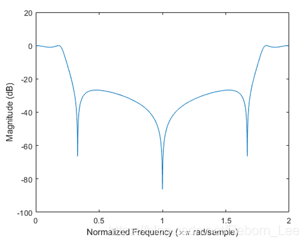
Compute and display the magnitude response of the third-order IIR lowpass filter described by the following transfer function:

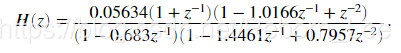
Express the numerator and denominator as polynomial convolutions. Find the frequency response at 2001 points spanning the complete unit circle.

clc;clear;close all;

b0 = 0.05634;
b1 = [1 1];
b2 = [1 -1.0166 1];
a1 = [1 -0.683];
a2 = [1 -1.4461 0.7957];

b = b0*conv(b1,b2);
a = conv(a1,a2);

[h,w] = freqz(b,a,'whole',2001);

% Plot the magnitude response expressed in decibels.


plot(w/pi,20*log10(abs(h)))
ax = gca;
ax.YLim = [-100 20];
ax.XTick = 0:.5:2;
xlabel('Normalized Frequency (\times\pi rad/sample)')
ylabel('Magnitude (dB)')

[h,w] = freqz(d,n) returns the n-point complex frequency response for the digital filter, d.

Frequency Response of an FIR Bandpass Filter

Design an FIR bandpass filter with passband between $0.35\pi$ and $0.8\pi$ rad/sample and 3 dB of ripple. The first stopband goes from 0 to $0.1\pi$ rad/sample and has an attenuation of 40 dB. The second stopband goes from $0.9\pi$ rad/sample to the Nyquist frequency and has an attenuation of 30 dB. Compute the frequency response. Plot its magnitude in both linear units and decibels. Highlight the passband.
sf1 = 0.1;
pf1 = 0.35;
pf2 = 0.8;
sf2 = 0.9;
pb = linspace(pf1,pf2,1e3)*pi;

bp = designfilt('bandpassfir', ...
'StopbandAttenuation1',40, 'StopbandFrequency1',sf1,...
'PassbandFrequency1',pf1,'PassbandRipple',3,'PassbandFrequency2',pf2, ...
'StopbandFrequency2',sf2,'StopbandAttenuation2',30);

[h,w] = freqz(bp,1024);
hpb = freqz(bp,pb);

subplot(2,1,1)
plot(w/pi,abs(h),pb/pi,abs(hpb),'.-')
axis([0 1 -1 2])
legend('Response','Passband','Location','South')
ylabel('Magnitude')

subplot(2,1,2)
plot(w/pi,db(h),pb/pi,db(hpb),'.-')
axis([0 1 -60 10])
xlabel('Normalized Frequency (\times\pi rad/sample)')
ylabel('Magnitude (dB)')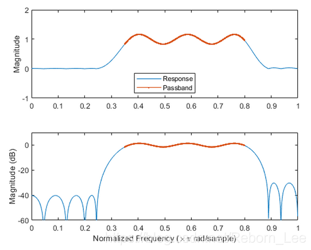

freqz(___) with no output arguments plots the frequency response of the filter.

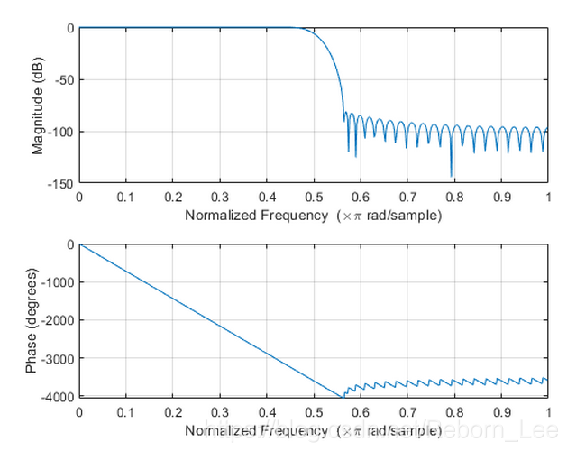
Frequency Response of an FIR filter

Design an FIR lowpass filter of order 80 using a Kaiser window with . Specify a normalized cutoff frequency of rad/sample. Display the magnitude and phase responses of the filter.

b = fir1(80,0.5,kaiser(81,8));
freqz(b,1)

Design the same filter using designfilt. Display its magnitude and phase responses using fvtool.
d = designfilt('lowpassfir','FilterOrder',80, ...
'CutoffFrequency',0.5,'Window',{'kaiser',8});
freqz(d)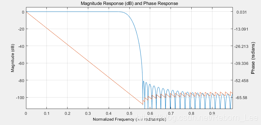

Note: If the input to freqz is single precision, the frequency response is calculated using single-precision arithmetic. The output, h, is single precision.

[h,w] = freqz(sos,n) returns the n-point complex frequency response corresponding to the second-order sections matrix, sos.

[h,f] = freqz(___,n,fs) returns the frequency response vector, h, and the corresponding physical frequency vector, f, for the digital filter with numerator and denominator polynomial coefficients stored in b and a, respectively, given the sample rate, fs.

[h,f] = freqz(___,n,'whole',fs) returns the frequency at n points ranging between 0 and fs.

h = freqz(___,w) returns the frequency response vector, h, at the normalized frequencies supplied in w.

h = freqz(___,f,fs) returns the frequency response vector, h, at the physical frequencies supplied in f.

【 MATLAB 】freqz 函数介绍（数字滤波器的频率响应）