def linear_plot():
    import numpy as np
    import matplotlib.pyplot as plt
    from sklearn.linear_model import LinearRegression
    data = [[5.06, 5.79], [4.92, 6.61], [4.67, 5.48], [4.54, 6.11], [4.26, 6.39],
            [4.07, 4.81], [4.01, 4.16], [4.01, 5.55], [3.66, 5.05], [3.43, 4.34],
            [3.12, 3.24], [3.02, 4.80], [2.87, 4.01], [2.64, 3.17], [2.48, 1.61],
            [2.48, 2.62], [2.02, 2.50], [1.95, 3.59], [1.79, 1.49], [1.54, 2.10]]
    data=np.array(data)
    x=np.array(data[:,0])
    y=np.array(data[:,1])
    fig=plt.figure()
    plt.scatter(x,y)
    x_mean = np.mean(x)
    y_mean = np.mean(y)

    up = np.sum((x - x_mean) * (y- y_mean))
    down = np.sum((x - x_mean) * (x - x_mean))
    w= up / down
    w=np.round(w,2)
    b= y_mean - w* x_mean
    b=np.round(b,2)
    plt.plot(x,w*x+b,c='red')
    fig.show()
    return w,b,fig

def linear_plot1():
    import numpy as np
    import matplotlib.pyplot as plt
    from sklearn.linear_model import LinearRegression
    data = [[5.06, 5.79], [4.92, 6.61], [4.67, 5.48], [4.54, 6.11], [4.26, 6.39],
            [4.07, 4.81], [4.01, 4.16], [4.01, 5.55], [3.66, 5.05], [3.43, 4.34],
            [3.12, 3.24], [3.02, 4.80], [2.87, 4.01], [2.64, 3.17], [2.48, 1.61],
            [2.48, 2.62], [2.02, 2.50], [1.95, 3.59], [1.79, 1.49], [1.54, 2.10]]
    data=np.array(data)
    x = np.array(data[:, 0])

    y=np.array(data[:,1])

    l=LinearRegression()

    l.fit(x.reshape(-1,1),y.reshape(-1,1))
    w=l.coef_
    b=l.intercept_
    w = np.round(w, 2)
    b = np.round(b, 2)

    y_predict = l.predict(x.reshape(-1,1))
    fig=plt.figure()
    plt.scatter(x,y)
    plt.plot(x,y_predict,c='r')
    plt.axis([0,7,0,8])
    plt.show()
    return w,b,fig
介绍
线性回归是机器学习中最基础、最重要的方法之一。接下来,你需要根据题目提供的数据点,完成线性拟合,并绘制出图像。
目标
题目给出一个二维数组如下,共计 20 个数据样本。
data = [[5.06, 5.79], [4.92, 6.61], [4.67, 5.48], [4.54, 6.11], [4.26, 6.39],
        [4.07, 4.81], [4.01, 4.16], [4.01, 5.55], [3.66, 5.05], [3.43, 4.34],
        [3.12, 3.24], [3.02, 4.80], [2.87, 4.01], [2.64, 3.17], [2.48, 1.61],
        [2.48, 2.62], [2.02, 2.50], [1.95, 3.59], [1.79, 1.49], [1.54, 2.10], ]
你需要根据这 20 个样本,使用线性回归拟合,得到自变量系数及截距项。
\displaystyle y(x, w) = wx + by(x,w)=wx+b
其中,ww 即为自变量系数,bb 则为常数项。
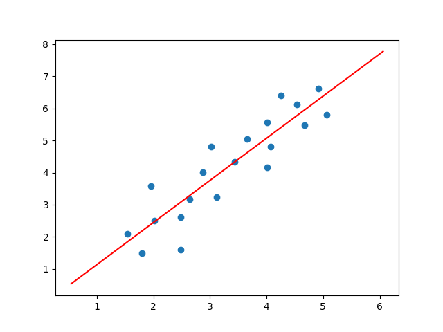
最后,需要使用 Matplotlib 将数据样本绘制成散点图,并将拟合直线一并绘出。
要求
全部代码写在
linear_plot()函数内部。计算出自变量系数 ww 及截距项 bb 的数值,保留两位小数(浮点数类型)并返回。
绘制出样本散点图,并根据参数将拟合直线绘于图中,最后返回绘图对象。
代码保存在
linear_regression.py文件中,并将该文件放置在/home/shiyanlou/Code路径下方。
提示
你可以使用自行实现的最小二乘法函数计算 ww 和 bb 的值,也可以使用 scikit-learn 提供的线性回归类完成。提示代码如下:
def linear_plot():
    """
    参数:无

    返回:
    w -- 自变量系数, 保留两位小数
    b -- 截距项, 保留两位小数
    fig -- matplotlib 绘图对象
    """

    data = [[5.06, 5.79], [4.92, 6.61], [4.67, 5.48], [4.54, 6.11], [4.26, 6.39],
            [4.07, 4.81], [4.01, 4.16], [4.01, 5.55], [3.66, 5.05], [3.43, 4.34],
            [3.12, 3.24], [3.02, 4.80], [2.87, 4.01], [2.64, 3.17], [2.48, 1.61],
            [2.48, 2.62], [2.02, 2.50], [1.95, 3.59], [1.79, 1.49], [1.54, 2.10], ]

    ### TODO: 线性拟合计算参数 ###

    w = None
    b = None

    fig = plt.figure() # 务必保留此行,设置绘图对象

    ### TODO: 按题目要求绘图 ###

    return w, b, fig # 务必按此顺序返回
如需使用 scikit-learn, Pandas 等第三方模块,可以通过 /home/shiyanlou/anaconda3/bin/python 路径执行。
图像示例:
知识点
- 线性回归拟合
- Matplotlib 绘图