目录
Abstract
As part of our approach, we propose a new reward shaping and devise a novel action space, from which a reinforcement learning agent can sample actions, which is independent of the job shop problem size.
作为我们的方法的一部分,我们提出了一个新的奖励塑造,并设计了一个新的行动空间,从一个强化学习智能体可以抽样行为,这是独立于加工车间。
- outperforms commonly used scheduling heuristics. 优于广泛应用的启发式调度算法。
- the time required to compute solutions using our methodology increases less sharply as the problem size grows. 计算时间会随着问题规模的增长仅产生较小幅度的增长。
Keywords
- Manufacturing Control
- Production Scheduling
- Job Shop Scheduling
- Deep Reinforcement Learning
- Combinatorial Optimization.
1 INTRODUCTION
While exact approaches such as integer linear programming (ILP) can be used to find optimal solutions, the time required to find such solutions is often impractical due to the NP-hardness of problems in this space.
虽然可以使用整数线性规划(ILP)等精确的方法来寻找最优解,但由于该空间中问题的np硬度,寻找最优解所需的时间往往是不切实际的
Should any of the underlying assumptions of the optimization problem change after the solution is created, these algorithms will have to create a complete solution once more, which again will result in a high cost in terms of computation time and render the application of such methods impractical in a dynamic production environment.
如果优化问题的任何基本假设在创建解决方案后发生变化,这些算法将不得不再次创建完整的解决方案,这将再次导致计算时间方面的高成本,并使此类方法在动态生产环境中的应用不切实际。
在这里,强化学习智能体一步一步地创建一个解决方案,而每一步都重新评估当前的情况,以便在智能体未来的决策过程中重新反映环境变化的新信息。
While this training is usually time-intensive, it only needs to be performed once and a trained agent can create scheduling solutions in reasonable time.
虽然这种培训通常是耗时的,但它只需要执行一次(训练),一个经过训练的智能体可以在合理的时间内创建调度解决方案。
没有数学保证以这种方式创建的解是最优的,但有一种可能性是,这种学习的启发式可以优于目前使用的启发式和优先级规则(保持低调度所需的时间)
强化学习的缺点:泛化到多种规则的车间调度问题的能力。
如果状态表示和动作空间直接与问题的大小相关联,即生产过程中的机器数量和订单数量,那么泛化只能在非常有限的程度上实现。
- 提出一种独立于机器数量和规划顺序的新的动作空间设计,能够推广到不同的问题规模
- 提出一种新的奖励塑造方法,通过高奖励梯度向最优方向激励接近最优调度策略的学习
2 BACKGROUND
2.1 Production Planning and Control
In general, the so-called logistical targets can be classified in logistical performance and logistical costs.
一般来说,所谓的后勤目标可以按后勤绩效和后勤成本进行分类。
The target of improving logistical performance can be further specified by shortening lead times and increasing the adherence to production schedules, both internally and externally.
通过缩短交货期和增加内部和外部对生产计划的遵守程度,可以进一步确定提高后勤绩效的目标。
On the other hand, the target of reducing logistical costs is expressed by increasing utilization of production resources and reducing work-in-process (WIP) and tied capital, subsequently.
另一方面,减少后勤成本的目标是通过增加生产资源的利用,随后减少进程中工作(WIP)和捆绑资本。
这些目标相互依赖,改进其中一个目标可能会导致其他目标的恶化。
例如,减少WIP可能会导致利用率的减少。
To approach these problems, manufacturing companies usually use software systems such as an enterprise resource planning (ERP) system.
The task of order release is to determine an optimal point in time to start with the production of an
order in a job shop production environment.
订单发布的任务是确定在工作车间生产环境中开始订单生产的最佳时间点。
在交货日期附近发布订单可以减少WIP和交货期,但会面临遵守交货日期较低的风险。
提前发布订单并不一定会导致更好地遵守交付日期,因为WIP的增加会导致更长、更分散的交货时间。
由于订单提前时间长达几周或几个月,PPC的第二个重要任务是在工作站进行订单排序。
排序的常见启发式方法是先入先出(FIFO)、设置时间优化或最小松弛。解决这个问题的进一步启发式方法是最短处理时间(SPT)和最长处理时间(LPT)优先级规则,在这些规则中,操作分别按处理时间的递增和递减的顺序进行排序。
2.2 Reinforcement Learning
A policy is learned with the goal of maximizing not the reward at any single time step, but rather the long-term cumulative reward.
策略目标不是在任何时间步最大化奖励,而是长期累积奖励
强化学习的简单分类(Review)
| Items | Contents |
|---|---|
| value-based | the value of each available action in a specific state is estimated and a policy is derived subsequently from these estimated values. |
| policy-based | a policy as described above is learned directly as a probability distribution of all actions in a given state. Such policy approaches typically update the learned policy at the end of an episode based on the overall reward received in that episode. Since actions are not evaluated individually, the current state of the policy might be evaluated as good overall while some of the actions performed where actually disadvantageous or vice versa. |
| a hybrid of value-based and policy-based approaches | allow for an evaluation of individual actions by updating the parameters of an actor, which is the policy-based component, based on the value estimates computed by a critic, which is the value-based component. |
In our work, we apply Deep Q-Learning (DQN) as an example of a value-based approach operating with discrete action spaces and Soft Actor-Critic (SAC) as a representative of the actor-critic group of algorithms relying on continuous action space design.
the function describing the long-term expected reward when performing action a a a in state s s s, is approximated.
Q ( s , a ) ← ( 1 − α ) Q ( s , a ) + α ( r + γ max a ∗ Q ( s ∗ , a ∗ ) ) Q(s,a) \leftarrow (1-\alpha) Q(s,a) + \alpha ( r+\gamma\max\limits_{a^{\ast}}Q(s^{\ast},a^{\ast}) ) Q(s,a)←(1−α)Q(s,a)+α(r+γa∗maxQ(s∗,a∗))
These networks improve by updating their parameters in the direction of the gradient of a so-called loss function, which compares the value Q ( s , a ) Q(s,a) Q(s,a) predicted by the network with the correct value.
In contrast to DQN, the SAC algorithm maximizes not just the expected reward but also the entropy of its policy, which promotes exploration and prevents premature convergence to local optima by encouraging the agent to act with as much randomness as possible while still succeeding at the given task.
与DQN相比,SAC算法不仅最大化了预期的奖励,还最大化了其策略的熵,通过鼓励智能体在给定任务的同时尽可能多地随机行动,促进了探索,并防止了过早收敛到局部最优。
3 RELATED WORK
强化学习用于调度问题包括以下几个方面
- 通过迭代,减少违反的数量来修改初始状态,但产生的是不可行的解
- 订单发布
- 根据当前状态选择适当的优先级规则来调度作业
- 多智能体方法在该领域尤其被研究。这可能是因为,当各种决策可以相互解耦并单独处理时,为这样的问题建模就会变得更容易。
- 在作业车间调度问题中,为每台机器分配一个单独的智能体
- 多智能体调度问题用于半导体生产设施
多智能体用于生产调度的困难在于:由于其他主体居住的环境的固有非平稳,训练这样一组代理往往更加困难。
由于单智能体的强化学习存在“状态空间和动作空间独立于机器数量和工作数量”的问题,作者通过引入一个独立于作业数量的行动空间来部分解决这个问题。
4 EXPERIMENTAL SETUP AND SOLUTION DESIGN
将强化学习应用于:订单发布和操作顺序。
即使是“3工作3机器”的问题,也具有较大的NP复杂度
4.1 Job-shop Problem Formalization
问题建模:
- 一系列的工作: J = { J 1 , J 2 , ⋯ , J n } J=\{ J_{1},J_{2},\cdots,J_{n} \} J={ J1,J2,⋯,Jn};
- 每项工作都有一系列的操作: J i , i = 1 , 2 , ⋯ , n J_{i},i=1,2,\cdots,n Ji,i=1,2,⋯,n且 O i = { O i 1 , O i 2 , ⋯ , O i n } O_{i}=\{ O_{i1},O_{i2},\cdots,O_{in} \} Oi={ Oi1,Oi2,⋯,Oin}。这些操作只能按照预先定义的顺序来进行。
- 每一个操作 O i , q , q = 1 , 2 , ⋯ , n O_{i,q},q=1,2,\cdots,n Oi,q,q=1,2,⋯,n 都有一个处理时间 t i , q t_{i,q} ti,q,且这个处理时间是非负性的。
- 有个机器集合 M = { M 1 , M 2 , ⋯ , M m } M=\{ M_{1},M_{2},\cdots,M_{m} \} M={ M1,M2,⋯,Mm},每个机器 M j , j = 1 , 2 , ⋯ , m M_{j},j=1,2,\cdots,m Mj,j=1,2,⋯,m,都能同时在一个操作 O i , q , q = 1 , 2 , ⋯ , n O_{i,q},q=1,2,\cdots,n Oi,q,q=1,2,⋯,n 上进行操作。
- 我们定义了优化目标,即:在 M M M 上找到一个时间表 J J J,以减少任何作业 J i J_{i} Ji 的最新结束时间,也称为最大限度的 C m a x C_{max} Cmax。
用MDP模型进行建模:
- 初始状态:在初始状态下,所有机器都空闲,生产程序中包含的订单放置在订单发布拉取中。
- 通过一组操作,强化学习智能体可以决定在一个时间单位内保持不活动,将订单从订单释放拉移到生产(订单释放),或将订单从一台机器移动到另一台机器(订单排序)。
- 当所有计划订单都完成,或强化学习智能体执行的操作数量超过预定义的限制时,将达到事件的最终状态。
- 使用稀疏奖励,这意味着奖励只在情节的最后一步给予,而所有中间步骤的奖励为零。这种稀疏的奖励与已实现的最长时间成反比。
4.2 RL Implementation
4.2.1 State Space Representation
智能体观察到的状态是由六个独立的组件组成:
- 机器状态,即剩余的时间操作目前正在处理的机器;在特定时间点的机器上没有处理作业,这个变量置为-1;
- 目前在每个机器的队列所有操作的处理时间的总和;
- 所有为每个单独的作业操作的处理时间的总和;
- 下一个操作的持续时间;如果不需要为一个特定的作业进行进一步的操作,则置为-1;
- 每个作业的下一个机器的指数;如果不需要为一个特定的作业进行进一步的操作,则置为-1;
- 时间已经在任何给定的时刻。
这些组件在传递到智能体之前都是标准化的。
4.2.2 Action Space Design
为了确保操作空间与每个作业的作业和操作数量不一致,智能体将选择将映射到特定操作的相对持续时间a,而不是直接选择该操作。
然后,由智能体选择的这种相对持续时间分别使用总体最小和最大处理时间 t m i n t_{min} tmin 和 t m a x t_{max} tmax映射回一个绝对持续时间。
然后将这个绝对持续时间与每个可用操作的处理时间 t i q t_{iq} tiq 进行比较,并选择与处理时间最近的操作 O s e l O_{sel} Osel,并形式化。
O s e l ← arg min i , q ( ∣ t i q − ( t m i n + a 10 × ( t m a x − t m i n ) ) ∣ ) O_{sel} \leftarrow \argmin\limits_{i,q}(|t_{iq}-(t_{min}+\frac{a}{10}\times(t_{max}-t_{min}))|) Osel←i,qargmin(∣tiq−(tmin+10a×(tmax−tmin))∣)
The proposed action space design allows for the use of RL agents with both discrete or continuous action space.
离散环境下是整数;连续环境下是实数;两者的范围都是在 [ − 1 , 10 ] [-1,10] [−1,10]。
正常情况是 [ 0 , 10 ] [0,10] [0,10],但是机器不运转的话就是 − 1 -1 −1。
4.2.3 Reward Shaping
虽然学习通常受益于更频繁的奖励,但在这种情况下,中间奖励是不同的定义方式,它们符合实际的优化目标,该目标只有在一个事件结束后才能被准确评估。
r ( T ) = 1000 × γ T O P T γ T r(T)=1000 \times \frac{\gamma^{T_{\mathbf{OPT}}}}{\gamma^{T}} r(T)=1000×γTγTOPT
4.3 Evaluation Approach
本研究的主要评价标准是解决方案质量、解决方案速度和对更大问题实例的可伸缩性。
与the OR-tools implementation of the CP-SAT solver、SPT和LPT进行对比
进行了三组实验: n n n machines, n n n jobs, n n n operations, n = 6 , 10 , 15 n=6,10,15 n=6,10,15
操作时间均一致地从 [ 1 , 11 ] [1,11] [1,11] 里面取出。
每个JSP实例都用CP-SAT、SPT和LPT求解器进行求解。
CP-SAT求解器发现的每个JSP实例的最大时间被认为是奖励计算的参考值,并在我们的研究中被用作性能基准。
解决方案质量被形式化为最优间隙(OptGap),可以被视为实现的最大值( T T T)和CP-SAT求解器( T o p t T_{opt} Topt)发现的参考最大间隔差异的函数。最优性间隙的值越低,对应的解就越好。
O p t G a p = T − T o p t T o p t × 100 OptGap = \frac{T −T_{opt}}{T_{opt}} \times 100 OptGap=ToptT−Topt×100
5 EXPERIMENTS AND RESULTS
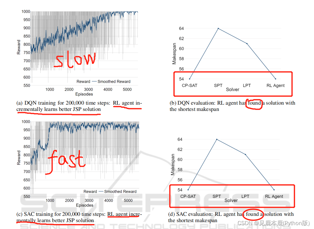
图2表明,新的动作空间设计同样适用于依赖于离散动作空间(如DQN)的RL智能体,以及在连续动作空间上操作的RL智能体(如SAC)。
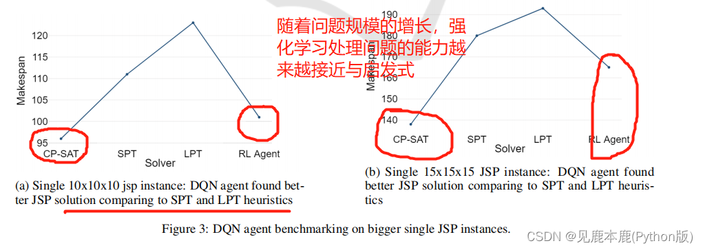
对于 10 × 10 × 10 10\times10\times10 10×10×10 和 15 × 15 × 15 15\times15\times15 15×15×15 的JSP,RL代理分别有 1500 , 000 1500,000 1500,000 和 2000 , 000 2000,000 2000,000 个时间步长,以逐步改进调度和调度策略。
随着JSP大小的增大,可以看到最优性差距的增大。
找到可行且接近最优的计划所需的较低运行时,增加了规划的灵活性,并允许尽量减少生产环境中意外变化和干扰的负面影响。
每次RL训练用不同的固定随机种子进行10次。
对RL智能体运行时的进一步分析表明,RL智能体基于给定的生产状态推断下一步所需的时间低于生产模拟环境中用于状态更新的计算时间的1%。