Residual Flows for Invertible Generative Modeling
Ricky T. Q. Chen 1,3 , Jens Behrmann 2 , David Duvenaud 1,3 , Jörn-Henrik Jacobsen 1,3 University of Toronto 1 , University of Bremen 2 , Vector Institute 3


[NeurIPS 2019] [github] [arxiv v2 (Appendix)] [arxiv v1 (Appendix)]
整篇文章理论性很强,感觉每一句话都浓缩了很重要的理论知识。
博主能力有限,只是将原文做了简单翻译和复述。建议感兴趣读者细读原文。
目录
3.1 Unbiased Log Density Estimation for Maximum Likelihood Estimation
3.2 Memory-Efficient Backpropagation
3.3 Avoiding Derivative Saturation with the LipSwish Activation
Abstract
Flow-based generative models parameterize probability distributions through an invertible transformation and can be trained by maximum likelihood. Invertible residual networks provide a flexible family of transformations where only Lipschitz conditions rather than strict architectural constraints are needed for enforcing invertibility. However, prior work trained invertible residual networks for density estimation by relying on biased log-density estimates whose bias increased with the network’s expressiveness.
We give a tractable unbiased estimate of the log density using a “Russian roulette” estimator, and reduce the memory required during training by using an alternative infinite series for the gradient. Furthermore, we improve invertible residual blocks by proposing the use of activation functions that avoid derivative saturation and generalizing the Lipschitz condition to induced mixed norms.
The resulting approach, called Residual Flows, achieves state-of-theart performance on density estimation amongst flow-based models, and outperforms networks that use coupling blocks at joint generative and discriminative modeling.
基于流的生成模型通过可逆变换参数化概率分布,并可以通过极大似然进行训练。可逆残差网络提供了一种灵活的变换家族,只需要 Lipschitz 条件而不是严格的结构约束就可以实现可逆性。然而,之前的工作是依靠有偏对数密度估计来训练可逆残差网络的密度估计,其偏差随着网络的表达性而增加。
本文使用 “俄罗斯轮盘赌” 估计器给出对数密度的一个易于处理的无偏估计,并通过使用一个可供选择的无穷级数的梯度来减少训练期间所需的记忆。进一步,提出了利用激活函数来避免导数饱和,并将 Lipschitz 条件推广到诱导混合范数,从而改进了可逆残块。
由此产生的方法,称为残差流,在基于流的模型中实现了密度估计的最新性能,并在联合生成和判别建模中优于使用耦合块的网络。
1 Introduction
Maximum likelihood is a core machine learning paradigm that poses learning as a distribution alignment problem. However, it is often unclear what family of distributions should be used to fit high-dimensional continuous data. In this regard, the change of variables theorem offers an appealing way to construct flexible distributions that allow tractable exact sampling and efficient evaluation of its density. This class of models is generally referred to as invertible or flow-based generative models (Deco and Brauer, 1995; Rezende and Mohamed, 2015).
With invertibility as its core design principle, flow-based models (also referred to as normalizing flows) have shown to be capable of generating realistic images (Kingma and Dhariwal, 2018) and can achieve density estimation performance on-par with competing state-of-the-art approaches (Ho et al., 2019). In applications, they have been applied to study adversarial robustness (Jacobsen et al., 2019) and are used to train hybrid models with both generative and classification capabilities (Nalisnick et al., 2019) using a weighted maximum likelihood objective.
研究背景:概念介绍及应用情况
最大似然是机器学习的核心范例,它将学习作为一个分布对齐问题。然而,通常不清楚应该使用哪种分布族来拟合高维连续数据。在这方面,变量变换定理提供了一种有吸引力的方法来构造灵活的分布,允许易于处理的精确抽样和其密度的有效评估。这类模型通常被称为可逆的或基于流的生成模型。
以可逆性为核心设计原则,基于流的模型 (也称为归一化流) 已经证明能够生成真实的图像,并可以实现与竞争的最先进方法相当的密度估计性能。在应用中,它们被用于研究对抗鲁棒性,并使用加权最大似然目标训练具有生成和分类能力的混合模型。
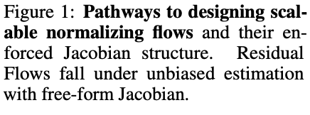
Existing flow-based models (Rezende and Mohamed, 2015; Kingma et al., 2016; Dinh et al., 2014; Chen et al., 2018) make use of restricted transformations with sparse or structured Jacobians (Figure 1). These allow efficient computation of the log probability under the model but at the cost of architectural engineering. Transformations that scale to high-dimensional data rely on specialized architectures such as coupling blocks (Dinh et al., 2014, 2017) or solving an ordinary differential equation (Grathwohl et al., 2019). Such approaches have a strong inductive bias that can hinder their application in other tasks, such as learning representations that are suitable for both generative and discriminative tasks.
提出问题:
现有的基于流的模型利用稀疏或结构化雅可比矩阵的限制性转换 (图1)。这允许在模型下高效地计算对数概率,但以结构工程为代价。可伸缩到高维数据的转换依赖于特殊的架构,如耦合块或求解常微分方程。这种方法有很强的归纳性偏差,可能会阻碍它们在其他任务中的应用,比如既适用于生成任务又适用于区别任务的学习表征。

Recent work by Behrmann et al. (2019) showed that residual networks (He et al., 2016) can be made invertible by simply enforcing a Lipschitz constraint, allowing to use a very successful discriminative deep network architecture for unsupervised flow-based modeling. Unfortunately, the density evaluation requires computing an infinite series.
The choice of a fixed truncation estimator used by Behrmann et al. (2019) leads to substantial bias that is tightly coupled with the expressiveness of the network, and cannot be said to be performing maximum likelihood as bias is introduced in the objective and gradients.
Behrmann et al. (2019) 最近的工作表明,残差网络可以通过简单地强制执行 Lipschitz 约束来实现可逆,允许使用非常成功的可识别深度网络体系结构进行无监督的基于流的建模。不幸的是,密度评估需要计算一个无穷级数。
Behrmann等人(2019)使用的固定截断估计器的选择导致了与网络的表达紧密耦合的大量偏差,不能说表现为最大似然,因为在目标和梯度中引入了偏差。
In this work, we introduce Residual Flows, a flow-based generative model that produces an unbiased estimate of the log density and has memory-efficient backpropagation through the log density computation. This allows us to use expressive architectures and train via maximum likelihood.
Furthermore, we propose and experiment with the use of activations functions that avoid derivative saturation and induced mixed norms for Lipschitz-constrained neural networks.
本文引入了残差流,一个基于流的生成模型,产生一个无偏估计的对数密度,并通过对数密度计算具有内存高效的反向传播。这允许我们使用表达架构,并通过最大可能性进行训练。此外,本文提出并实验使用激活函数,以避免导数饱和和诱导混合规范的 Lipschitz 约束神经网络。
2 Background
Maximum likelihood estimation
To perform maximum likelihood with stochastic gradient descent, it is sufficient to have an unbiased estimator for the gradient as
where p_data is the unknown data distribution which can be sampled from and p_θ is the model distribution. An unbiased estimator of the gradient also immediately follows from an unbiased estimator of the log density function, log p_θ(x).
最大似然估计
要用随机梯度下降法进行极大似然估计,只要有一个无偏估计就足够了,如(1)。
其中 p_data 为可抽样的未知数据分布,p_θ 为模型分布。梯度的无偏估计也紧跟着对数密度函数(log p_θ(x)) 的无偏估计。
Change of variables theorem
With an invertible transformation f, the change of variables
captures the change in density of the transformed samples. A simple base distribution such as a standard normal is often used for log p(f(x)). Tractable evaluation of (2) allows flow-based models to be trained using the maximum likelihood objective (1). In contrast, variational autoencoders (Kingma and Welling, 2014) can only optimize a stochastic lower bound, and generative adversial networks (Goodfellow et al., 2014) require an extra discriminator network for training.
变量变换定理
对于可逆变换 f,也就是变量的变换 (2),捕获转换后样本的密度变化。log p(f(x)) 通常使用简单的基数分布,如标准正态分布。(2) 的可处理性评估允许使用最大似然目标 (1) 来训练基于流模型。相反,变分自编码器只能优化随机下界,而生成对抗网络需要额外的鉴别器网络来训练。
Invertible residual networks (i-ResNets)
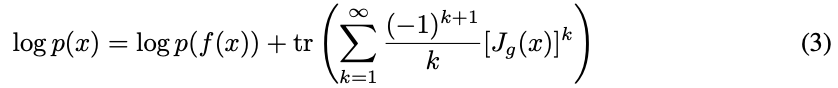
Residual networks are composed of simple transformations y = f(x) = x + g(x). Behrmann et al. (2019) noted that this transformation is invertible by the Banach fixed point theorem if g is contractive, i.e. with Lipschitz constant strictly less than unity, which was enforced using spectral normalization (Miyato et al., 2018; Gouk et al., 2018). Applying i-ResNets to the change-of-variables (2), the identity
was shown, where Jg(x) = dg(x)/dx . Furthermore, the Skilling-Hutchinson estimator (Skilling, 1989; Hutchinson, 1990) was used to estimate the trace in the power series. Behrmann et al. (2019) used a fixed truncation to approximate the infinite series in (3). However, this naïve approach has a bias that grows with the number of dimensions of x and the Lipschitz constant of g, as both affect the convergence rate of this power series. As such, the fixed truncation estimator requires a careful balance between bias and expressiveness, and cannot scale to higher dimensional data. Without decoupling the objective and estimation bias, i-ResNets end up optimizing for the bias without improving the actual maximum likelihood objective (see Figure 2).
可逆残差网络 (i-ResNets)
残差网络由简单变换 y = f(x) = x + g(x) 组成。Behrmann et al. (2019) 指出,如果 g 是收缩的,即 Lipschitz 常数严格小于单位时,这种变换可通过 Banach 不动点定理实现可逆。将 i-ResNets 应用于变量的变更 (2),得到恒等式(3),其中 Jg(x) = dg(x)/dx。
此外,斯基林-哈钦森估计量被用来估计幂级数的轨迹。Behrmann et al. (2019) 使用固定的截断来近似 (3) 中的无穷级数。然而,naïve 方法有一个偏差,随着 x 的维数和 g 的 Lipschitz 常数的增加而增加,因为两者都会影响幂级数的收敛速度。因此,固定的截断估计器需要偏差和表达之间的谨慎平衡,而不能扩展到更高维度的数据。在不将目标和估计偏差解耦的情况下,i-ResNets 最终会优化偏差,而不会改善实际的最大似然目标 (见图 2)。

Figure 2: i-ResNets suffer from substantial bias when using expressive networks, whereas Residual Flows principledly perform maximum likelihood with unbiased stochastic gradients.
3 Residual Flows
3.1 Unbiased Log Density Estimation for Maximum Likelihood Estimation
最大似然估计的无偏对数密度估计
Evaluation of the exact log density function log pθ(·) in (3) requires infinite time due to the power series. Instead, we rely on randomization to derive an unbiased estimator that can be computed in finite time (with probability one) based on an existing concept (Kahn, 1955).
问题:(3) 中对数密度函数 的精确计算由于幂级数的关系需要无限长的时间。相反,本文依靠随机化来推导一个无偏估计量,该估计量可以基于现有概念在有限时间内 (概率为1) 计算出来。
To illustrate the idea, let ∆k denote the k-th term of an infinite series, and suppose we always evaluate the first term then flip a coin b ∼ Bernoulli(q) to determine whether we stop or continue evaluating the remaining terms. By reweighting the remaining terms by 1/(1−q), we obtain an unbiased estimator
为了说明这个想法,令 ∆k 表示无穷级数的第 k 项,并假设总是计算第一项,然后抛一个硬币 b ~ Bernoulli(q) 来决定是停止还是继续计算剩下的项。通过用 1/(1−q) 重新加权其余项,得到一个无偏估计器。
Interestingly, whereas naïve computation would always use infinite compute, this unbiased estimator has probability q of being evaluated in finite time. We can obtain an estimator that is evaluated in finite time with probability one by applying this process infinitely many times to the remaining terms. Directly sampling the number of evaluated terms, we obtain the appropriately named “Russian roulette” estimator (Kahn, 1955)
有趣的是,naïve 计算总是使用无限计算,这个无偏估计器有概率为 q 的可能中有限时间内被计算的。本文可以得到一个在概率为 1 的可能中有限时间内的估计器,将这个过程无限次地应用到剩余的项上。直接抽样评估项的数量,命名为 “俄罗斯轮盘赌” 估计量。
We note that the explanation above is only meant to be an intuitive guide and not a formal derivation. The peculiarities of dealing with infinite quantities dictate that we must make assumptions on ∆k, p(N), or both in order for the equality in (5) to hold. While many existing works have made different assumptions depending on specific applications of (5), we state our result as a theorem where the only condition is that p(N) must have support over all of the indices.
注意到上面的解释只是一种直观的指导,而不是一种形式的推导。处理无限量的特性要求必须对∆k, p(N),或两者都做假设,以便 (5) 中的等式成立。虽然许多现有的著作根据 (5) 的具体应用做出了不同的假设,但本文将我们的结果表述为一个定理,其中唯一的条件是 p(N) 必须支持所有的指标。
_____________________________________________________________________
_____________________________________________________________________
Here we have used the Skilling-Hutchinson trace estimator (Skilling, 1989; Hutchinson, 1990) to estimate the trace of the matrices
. A detailed proof is given in Appendix B.
Note that since Jg is constrained to have a spectral radius less than unity, the power series converges exponentially. The variance of the Russian roulette estimator is small when the infinite series exhibits fast convergence (Rhee and Glynn, 2015; Beatson and Adams, 2019), and in practice, we did not have to tune p(N) for variance reduction. Instead, in our experiments, we compute two terms exactly and then use the unbiased estimator on the remaining terms with a single sample from p(N) = Geom(0.5). This results in an expected compute cost of 4 terms, which is less than the 5 to 10 terms that Behrmann et al. (2019) used for their biased estimator.
Theorem 1 forms the core of Residual Flows, as we can now perform maximum likelihood training by backpropagating through (6) to obtain unbiased gradients. This allows us to train more expressive networks where a biased estimator would fail (Figure 2). The price we pay for the unbiased estimator is variable compute and memory, as each sample of the log density uses a random number of terms in the power series.
_____________________________________________________________________
定理1 (无偏对数密度估计)。设 f(x) = x + g(x), Lip(g) < 1, N 是一个支持正整数的随机变量。
则:![]() ,其中 n ∼ p(N) 且 v ∼ N (0, I). _____________________________________________________________________
,其中 n ∼ p(N) 且 v ∼ N (0, I). _____________________________________________________________________
这里使用了斯基林-哈钦森迹估计器估计矩阵 的迹。详细的证明参见附录 B。
注意,由于Jg 的谱半径小于单位,幂级数以指数形式收敛。当无穷级数呈现快速收敛时,俄罗斯轮盘赌估计量的方差很小,在实践中,不必调整 p(N) 来减少方差。相反,在实验中,我们精确地计算两项,然后使用一个样本 p(N) = Geom(0.5) 对其余项的无偏估计量。这导致预期的计算成本为 4 项,小于 Behrmann et al. (2019) 用于有偏估计的 5 至 10 项。
定理 1 形成了残差流的核心,因为该定理说明可以通过反向传播 (6) 来执行最大似然训练,以获得无偏梯度。这允许在有偏估计器失败的情况下训练更有表现力的网络 (图 2)。我们为无偏估计器付出的代价是变量计算和内存,因为对数密度的每个样本使用幂级数中的随机数。
Figure 2: i-ResNets suffer from substantial bias when using expressive networks, whereas Residual Flows principledly perform maximum likelihood with unbiased stochastic gradients.
3.2 Memory-Efficient Backpropagation
Memory can be a scarce resource, and running out of memory due to a large sample from the unbiased estimator can halt training unexpectedly. To this end, we propose two methods to reduce the memory consumption during training.
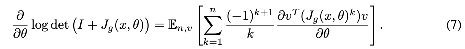
To see how naïve backpropagation can be problematic, the gradient w.r.t. parameters θ by directly differentiating through the power series (6) can be expressed as
Unfortunately, this estimator requires each term to be stored in memory because ∂/∂θ needs to be applied to each term. The total memory cost is then O(n · m) where n is the number of computed terms and m is the number of residual blocks in the entire network. This is extremely memory-hungry during training, and a large random sample of n can occasionally result in running out of memory.
节约内存反向传播
内存是一种稀缺资源,由于无偏估计量的大样本而耗尽内存会意外地停止训练。为此,本文提出了两种减少训练中记忆消耗的方法。
为了了解 naïve 的反向传播是如何有问题的,直接通过幂级数 (6) 微分的梯度 w.r.t. 参数 θ 可以表示为 (7)。
不幸的是,这个估计器需要将每个项存储在内存中,因为∂/∂θ需要应用于每个项。则总存储代价为O(n·m),其中 n 为计算项的个数,m 为整个网络中残差块的个数。这在训练过程中是非常需要记忆的,大量的随机样本 n 偶尔会导致内存耗尽。
Neumann gradient series
Instead, we can specifically express the gradients as a power series derived from a Neumann series (see Appendix C). Applying the Russian roulette and trace estimators, we obtain the following theorem.
________________________________________________________________________
_______________________________________________________________________
As the power series in (8) does not need to be differentiated through, using this reduces the memory requirement by a factor of n. This is especially useful when using the unbiased estimator as the memory will be constant regardless of the number of terms we draw from p(N).

方法一:诺伊曼梯度序列
相反,可以将梯度具体表示为由 Neumann 级数导出的幂级数 (见附录C)。应用俄罗斯轮盘赌和跟踪估计,得到以下定理。
—————————————————————————————————————————
定理 2 (无偏对数行列式梯度估计)。设Lip(g) < 1, N是支持正整数的随机变量。则:
![]() ,其中 n ∼ p(N) 且 v ∼ N (0, I)。
,其中 n ∼ p(N) 且 v ∼ N (0, I)。
—————————————————————————————————————————
由于(8)中的幂级数不需要对其进行微分,因此使用该方法可将内存需求减少n倍。当使用无偏估计器时,这尤其有用,因为无论我们从p(n)中提取的项的数量如何,内存都是常数。
Backward-in-forward: early computation of gradients
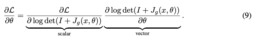
We can further reduce memory by partially performing backpropagation during the forward evaluation. By taking advantage of log det(I + Jg(x, θ)) being a scalar quantity, the partial derivative from the objective L is
For every residual block, we compute ∂ log det(I+Jg(x,θ))/∂θ along with the forward pass, release the memory for the computation graph, then simply multiply by ∂L/∂ log det(I+Jg(x,θ)) later during the main backprop. This reduces memory by another factor of m to O(1) with negligible overhead.
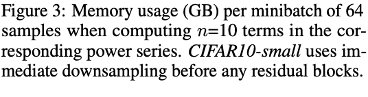
Note that while these two tricks remove the memory cost from backpropagating through the log det terms, computing the path-wise derivatives from log p(f(x)) still requires the same amount of memory as a single evaluation of the residual network. Figure 3 shows that the memory consumption can be enormous for naïve backpropagation, and using large networks would have been intractable.
方法二:向后向前,梯度的早期计算
可以通过在正向求值时部分执行反向传播来进一步减少内存。利用对数 det(I + Jg(x, θ)) 是一个标量,对目标 L 的偏导数为(9)。
对于每个残差块,计算 ∂log det(I+Jg(x, θ))/∂θ,随着向前传递,释放计算图的内存,然后在主支撑期间简单地乘以 ∂L/∂log det(I+Jg(x, θ))。这将内存减少 m 到 O(1) 的另一个因数,开销可以忽略不计。
注意,虽然这两种方法消除了通过对数 det 项反向传播的内存成本,但计算 log p(f(x)) 的路径导数仍然需要与残差网络的单个评估相同的内存量。图 3 显示了 naïve 反向传播的内存消耗可能是巨大的,使用大型网络可能是难以处理的。

3.3 Avoiding Derivative Saturation with the LipSwish Activation
Function As the log density depends on the first derivatives through the Jacobian Jg, the gradients for training depend on second derivatives. Similar to the phenomenon of saturated activation functions, Lipschitzconstrained activation functions can have a derivative saturation problem. For instance, the ELU activation used by Behrmann et al. (2019) achieves the highest Lipschitz constant when ELU0 (z) = 1, but this occurs when the second derivative is exactly zero in a very large region, implying there is a trade-off between a large Lipschitz constant and non-vanishing gradients.
We thus desire two properties from our activation functions φ(z):
1. The first derivatives must be bounded as |φ 0 (z)| ≤ 1 for all z;
2. The second derivatives should not asymptotically vanish when |φ 0 (z)| is close to one.
While many activation functions satisfy condition 1, most do not satisfy condition 2. We argue that the ELU and softplus activations are suboptimal due to derivative saturation. Figure 4 shows that when softplus and ELU saturate at regions of unit Lipschitz, the second derivative goes to zero, which can lead to vanishing gradients during training.
使用 LipSwish 激活避免导数饱和
由于对数密度依赖于雅可比矩阵 Jg 的一阶导数,所以用于训练的梯度依赖于二阶导数。与饱和激活函数现象相似,Lipschitz 约束激活函数也会出现导数饱和问题。例如,Behrmann et al. (2019)使用的 ELU 激活在 ELU'(z) = 1时达到最高的 Lipschitz常 数,但这发生在二阶导数在一个非常大的区域恰好为零时,这意味着在大的 Lipschitz 常数和非消失梯度之间存在折衷。
因此,我们希望激活函数 φ(z) 具有两个性质:
1. 对于所有 z,一阶导数必须有界为 |φ'(z)|≤1;
2. 当 |φ'(z)| 接近 1 时,二阶导数不应渐近消失。
虽然许多激活函数满足条件 1,但大多数不满足条件 2。我们认为,由于导数饱和,ELU 和softplus 激活是次优的。从图 4 可以看出,当 softplus 和 ELU 在单元 Lipschitz 区域饱和时,二阶导数趋于零,这会导致训练时梯度消失。

We find that good activation functions satisfying condition 2 are smooth and non-monotonic functions, such as Swish (Ramachandran et al., 2017). However, Swish by default does not satisfy condition 1 as
. But scaling via
where σ is the sigmoid function, results in
for all values of β. LipSwish is a simple modification to Swish that exhibits a less than unity Lipschitz property. In our experiments, we parameterize β to be strictly positive by passing it through softplus. Figure 4 shows that in the region of maximal Lipschitz, LipSwish does not saturate due to its non-monotonicity property.
本文发现满足条件 2 的良好激活函数是光滑的非单调函数,如 Swish。然而,Swish 默认不满足条件 1 为 。但通过扩展 (10),其中 σ 为 sigmoid 函数,对于所有 β 值,
。LipSwish 是 Swish 的一个简单修改,它展示了一个小于统一的Lipschitz 属性。在实验中,通过软加参数使 β 严格为正。从图 4 可以看出,在极大的 Lipschitz 区域,LipSwish 由于其非单调性而不饱和。