官方的API参考文档: https://pandas.pydata.org/docs/reference/index.html
可以简单的了解一个pandas,以后需要使用再查文档也不迟
import pandas as pd
API文档中显示pandas可以读取三种格式的文档,如下所示:
read_table(filepath_or_buffer[, sep, …])
Read general delimited file into DataFrame.
read_csv(filepath_or_buffer[, sep, …])
Read a comma-separated values (csv) file into DataFrame.
read_fwf(filepath_or_buffer[, colspecs, …])
Read a table of fixed-width formatted lines into DataFrame.
df = pd. read_csv( './data/titanic.csv' )
df. head( )
PassengerId
Survived
Pclass
Name
Sex
Age
SibSp
Parch
Ticket
Fare
Cabin
Embarked
0
1
0
3
Braund, Mr. Owen Harris
male
22.0
1
0
A/5 21171
7.2500
NaN
S
1
2
1
1
Cumings, Mrs. John Bradley (Florence Briggs Th...
female
38.0
1
0
PC 17599
71.2833
C85
C
2
3
1
3
Heikkinen, Miss. Laina
female
26.0
0
0
STON/O2. 3101282
7.9250
NaN
S
3
4
1
1
Futrelle, Mrs. Jacques Heath (Lily May Peel)
female
35.0
1
0
113803
53.1000
C123
S
4
5
0
3
Allen, Mr. William Henry
male
35.0
0
0
373450
8.0500
NaN
S
df. tail( )
PassengerId
Survived
Pclass
Name
Sex
Age
SibSp
Parch
Ticket
Fare
Cabin
Embarked
886
887
0
2
Montvila, Rev. Juozas
male
27.0
0
0
211536
13.00
NaN
S
887
888
1
1
Graham, Miss. Margaret Edith
female
19.0
0
0
112053
30.00
B42
S
888
889
0
3
Johnston, Miss. Catherine Helen "Carrie"
female
NaN
1
2
W./C. 6607
23.45
NaN
S
889
890
1
1
Behr, Mr. Karl Howell
male
26.0
0
0
111369
30.00
C148
C
890
891
0
3
Dooley, Mr. Patrick
male
32.0
0
0
370376
7.75
NaN
Q
指定读取数据返回结果的名字叫做df,其实就是pandas工具包中最常用的基础结构DataFrame结构
df. info( )
<class 'pandas.core.frame.DataFrame'>
RangeIndex: 891 entries, 0 to 890
Data columns (total 12 columns):
 #   Column       Non-Null Count  Dtype
---  ------       --------------  -----
 0   PassengerId  891 non-null    int64
 1   Survived     891 non-null    int64
 2   Pclass       891 non-null    int64
 3   Name         891 non-null    object
 4   Sex          891 non-null    object
 5   Age          714 non-null    float64
 6   SibSp        891 non-null    int64
 7   Parch        891 non-null    int64
 8   Ticket       891 non-null    object
 9   Fare         891 non-null    float64
 10  Cabin        204 non-null    object
 11  Embarked     889 non-null    object
dtypes: float64(2), int64(5), object(5)
memory usage: 83.7+ KB
DataFrame的其他属性
df. index
RangeIndex(start=0, stop=891, step=1)
df. columns
Index(['PassengerId', 'Survived', 'Pclass', 'Name', 'Sex', 'Age', 'SibSp',
       'Parch', 'Ticket', 'Fare', 'Cabin', 'Embarked'],
      dtype='object')
df. dtypes
PassengerId      int64
Survived         int64
Pclass           int64
Name            object
Sex             object
Age            float64
SibSp            int64
Parch            int64
Ticket          object
Fare           float64
Cabin           object
Embarked        object
dtype: object
df. values
array([[1, 0, 3, ..., 7.25, nan, 'S'],
       [2, 1, 1, ..., 71.2833, 'C85', 'C'],
       [3, 1, 3, ..., 7.925, nan, 'S'],
       ...,
       [889, 0, 3, ..., 23.45, nan, 'S'],
       [890, 1, 1, ..., 30.0, 'C148', 'C'],
       [891, 0, 3, ..., 7.75, nan, 'Q']], dtype=object)
age = df[ 'Age' ]
print ( "single:\n" , age[ 0 ] )
print ( "more:\n" , age[ : 5 ] )
age. values[ : 5 ]
single:
 22.0
more:
 0    22.0
1    38.0
2    26.0
3    35.0
4    35.0
Name: Age, dtype: float64


array([22., 38., 26., 35., 35.])
一般情况下是用数字来作为索引的,但还可以将其他内容设置为索引,比如所名字设置为索引
df. head( )
PassengerId
Survived
Pclass
Name
Sex
Age
SibSp
Parch
Ticket
Fare
Cabin
Embarked
0
1
0
3
Braund, Mr. Owen Harris
male
22.0
1
0
A/5 21171
7.2500
NaN
S
1
2
1
1
Cumings, Mrs. John Bradley (Florence Briggs Th...
female
38.0
1
0
PC 17599
71.2833
C85
C
2
3
1
3
Heikkinen, Miss. Laina
female
26.0
0
0
STON/O2. 3101282
7.9250
NaN
S
3
4
1
1
Futrelle, Mrs. Jacques Heath (Lily May Peel)
female
35.0
1
0
113803
53.1000
C123
S
4
5
0
3
Allen, Mr. William Henry
male
35.0
0
0
373450
8.0500
NaN
S
df = df. set_index( 'Name' )
df. head( )
PassengerId
Survived
Pclass
Sex
Age
SibSp
Parch
Ticket
Fare
Cabin
Embarked
Name
Braund, Mr. Owen Harris
1
0
3
male
22.0
1
0
A/5 21171
7.2500
NaN
S
Cumings, Mrs. John Bradley (Florence Briggs Thayer)
2
1
1
female
38.0
1
0
PC 17599
71.2833
C85
C
Heikkinen, Miss. Laina
3
1
3
female
26.0
0
0
STON/O2. 3101282
7.9250
NaN
S
Futrelle, Mrs. Jacques Heath (Lily May Peel)
4
1
1
female
35.0
1
0
113803
53.1000
C123
S
Allen, Mr. William Henry
5
0
3
male
35.0
0
0
373450
8.0500
NaN
S
age = df[ 'Age' ]
print ( "Braund, Mr. Owen Harris age:" , age[ 'Braund, Mr. Owen Harris' ] )
print ( "Futrelle, Mrs. Jacques Heath (Lily May Peel) age:" , age[ 'Futrelle, Mrs. Jacques Heath (Lily May Peel)' ] )
Braund, Mr. Owen Harris age: 22.0
Futrelle, Mrs. Jacques Heath (Lily May Peel) age: 35.0
df = df. reset_index( )
Clichong = df[ [ 'Name' , 'Age' , 'Fare' ] ]
Clichong[ : 5 ]
Name
Age
Fare
0
Braund, Mr. Owen Harris
22.0
7.2500
1
Cumings, Mrs. John Bradley (Florence Briggs Th...
38.0
71.2833
2
Heikkinen, Miss. Laina
26.0
7.9250
3
Futrelle, Mrs. Jacques Heath (Lily May Peel)
35.0
53.1000
4
Allen, Mr. William Henry
35.0
8.0500
索引中可以使用iloc函数或者是loc函数来取索引,以iloc为例
print ( "df.iloc[2]" , df. iloc[ 2 ] )
print ( "\n df.iloc[1:4]" , df. iloc[ 1 : 4 ] )
print ( "\n df.iloc[1:4,1:3]" , df. iloc[ 1 : 4 , 1 : 3 ] )
df.iloc[2] index                               2
Name           Heikkinen, Miss. Laina
PassengerId                         3
Survived                            1
Pclass                              3
Sex                            female
Age                                26
SibSp                               0
Parch                               0
Ticket               STON/O2. 3101282
Fare                            7.925
Cabin                             NaN
Embarked                            S
Name: 2, dtype: object

 df.iloc[1:4]    index                                               Name  PassengerId  \
1      1  Cumings, Mrs. John Bradley (Florence Briggs Th...            2
2      2                             Heikkinen, Miss. Laina            3
3      3       Futrelle, Mrs. Jacques Heath (Lily May Peel)            4

   Survived  Pclass     Sex   Age  SibSp  Parch            Ticket     Fare  \
1         1       1  female  38.0      1      0          PC 17599  71.2833
2         1       3  female  26.0      0      0  STON/O2. 3101282   7.9250
3         1       1  female  35.0      1      0            113803  53.1000

  Cabin Embarked
1   C85        C
2   NaN        S
3  C123        S

 df.iloc[1:4,1:3]                                                 Name  PassengerId
1  Cumings, Mrs. John Bradley (Florence Briggs Th...            2
2                             Heikkinen, Miss. Laina            3
3       Futrelle, Mrs. Jacques Heath (Lily May Peel)            4
df. loc[ 2 ]
Name           Heikkinen, Miss. Laina
index                               2
PassengerId                         3
Survived                            1
Pclass                              3
Sex                            female
Age                                26
SibSp                               0
Parch                               0
Ticket               STON/O2. 3101282
Fare                            7.925
Cabin                             NaN
Embarked                            S
Name: 2, dtype: object
df. loc[ 2 , 'Sex' ]
'female'
df. loc[ 0 : 2 ]
Name
index
PassengerId
Survived
Pclass
Sex
Age
SibSp
Parch
Ticket
Fare
Cabin
Embarked
0
Braund, Mr. Owen Harris
0
1
0
3
male
22.0
1
0
A/5 21171
7.2500
NaN
S
1
Cumings, Mrs. John Bradley (Florence Briggs Th...
1
2
1
1
female
38.0
1
0
PC 17599
71.2833
C85
C
2
Heikkinen, Miss. Laina
2
3
1
3
female
26.0
0
0
STON/O2. 3101282
7.9250
NaN
S
df. loc[ 0 : 2 , 'Name' ]
0                              Braund, Mr. Owen Harris
1    Cumings, Mrs. John Bradley (Florence Briggs Th...
2                               Heikkinen, Miss. Laina
Name: Name, dtype: object
df = df. set_index( 'Name' )
df[ 'Sex' ] == 'male'
Name
Braund, Mr. Owen Harris                                 True
Cumings, Mrs. John Bradley (Florence Briggs Thayer)    False
Heikkinen, Miss. Laina                                 False
Futrelle, Mrs. Jacques Heath (Lily May Peel)           False
Allen, Mr. William Henry                                True
                                                       ...
Montvila, Rev. Juozas                                   True
Graham, Miss. Margaret Edith                           False
Johnston, Miss. Catherine Helen "Carrie"               False
Behr, Mr. Karl Howell                                   True
Dooley, Mr. Patrick                                     True
Name: Sex, Length: 891, dtype: bool
df[ df[ 'Sex' ] == 'male' ] [ 0 : 5 ]
PassengerId
Survived
Pclass
Sex
Age
SibSp
Parch
Ticket
Fare
Cabin
Embarked
Name
Braund, Mr. Owen Harris
1
0
3
male
22.0
1
0
A/5 21171
7.2500
NaN
S
Allen, Mr. William Henry
5
0
3
male
35.0
0
0
373450
8.0500
NaN
S
Moran, Mr. James
6
0
3
male
NaN
0
0
330877
8.4583
NaN
Q
McCarthy, Mr. Timothy J
7
0
1
male
54.0
0
0
17463
51.8625
E46
S
Palsson, Master. Gosta Leonard
8
0
3
male
2.0
3
1
349909
21.0750
NaN
S
df. loc[ df[ 'Sex' ] == 'male' , 'Age' ] . mean( )
0      22.0
4      35.0
5       NaN
6      54.0
7       2.0
       ...
883    28.0
884    25.0
886    27.0
889    26.0
890    32.0
Name: Age, Length: 577, dtype: float64
df[‘Sex’] == ‘male’ :为晒选出男性
df.loc[df[‘Sex’] == ‘male’,‘Age’] :列举出全部男性的年龄
df.loc[df[‘Sex’] == ‘male’,‘Age’].mean : 求出平均年龄
df[ df[ 'Age' ] >= 70 ]
Name
PassengerId
Survived
Pclass
Sex
Age
SibSp
Parch
Ticket
Fare
Cabin
Embarked
96
Goldschmidt, Mr. George B
97
0
1
male
71.0
0
0
PC 17754
34.6542
A5
C
116
Connors, Mr. Patrick
117
0
3
male
70.5
0
0
370369
7.7500
NaN
Q
493
Artagaveytia, Mr. Ramon
494
0
1
male
71.0
0
0
PC 17609
49.5042
NaN
C
630
Barkworth, Mr. Algernon Henry Wilson
631
1
1
male
80.0
0
0
27042
30.0000
A23
S
672
Mitchell, Mr. Henry Michael
673
0
2
male
70.0
0
0
C.A. 24580
10.5000
NaN
S
745
Crosby, Capt. Edward Gifford
746
0
1
male
70.0
1
1
WE/P 5735
71.0000
B22
S
851
Svensson, Mr. Johan
852
0
3
male
74.0
0
0
347060
7.7750
NaN
S
( df[ 'Age' ] >= 70 ) . sum ( )
7
df. loc[ df[ 'Age' ] >= 70 , 'Age' ] . sum ( )
506.5
创建DataFrame
data = {
'country' : [ 'China' , 'America' , 'India' ] , 'population' : [ 14 , 5 , 25 ] }
df = pd. DataFrame( data)
df
country
population
0
China
14
1
America
5
2
India
25
df[ df[ 'population' ] >= 14 ]
country
population
0
China
14
2
India
25
参数设置 set_option
pd. set_option( 'display.max_rows' , 6 )
df
PassengerId
Survived
Pclass
Name
Sex
Age
SibSp
Parch
Ticket
Fare
Cabin
Embarked
0
1
0
3
Braund, Mr. Owen Harris
male
22.0
1
0
A/5 21171
7.2500
NaN
S
1
2
1
1
Cumings, Mrs. John Bradley (Florence Briggs Th...
female
38.0
1
0
PC 17599
71.2833
C85
C
2
3
1
3
Heikkinen, Miss. Laina
female
26.0
0
0
STON/O2. 3101282
7.9250
NaN
S
...
...
...
...
...
...
...
...
...
...
...
...
...
888
889
0
3
Johnston, Miss. Catherine Helen "Carrie"
female
NaN
1
2
W./C. 6607
23.4500
NaN
S
889
890
1
1
Behr, Mr. Karl Howell
male
26.0
0
0
111369
30.0000
C148
C
890
891
0
3
Dooley, Mr. Patrick
male
32.0
0
0
370376
7.7500
NaN
Q
891 rows × 12 columns
print ( "pd.get_option('display.max_rows'):" , pd. get_option( 'display.max_rows' ) )
print ( "pd.get_option('display.max_columns'):" , pd. get_option( 'display.max_columns' ) )
pd.get_option('display.max_rows'): 6
pd.get_option('display.max_columns'): 20
读取数据都是二维的,也就是DataFrame结构,而如果在数据中单独取某一列数据,那就是Series格式了。
相当于DataFrame结构是有Series组合起来得到的,因而会更高级一点
data = [ 1 , 2 , 3 ]
index = [ 'a' , 'b' , 'c' ]
Clichong = pd. Series( data = data, index = index)
Clichong
a    1
b    2
c    3
dtype: int64
Clichong. loc[ 'b' ]
2
Clichong. iloc[ 1 ]
2
Clichong_cp = Clichong. copy( )
Clichong_cp[ 'b' ]
2
Clichong. replace( to_replace= 1 , value= 100 , inplace= True )
Clichong
a    100
b      2
c      3
dtype: int64
Clichong. index
Index(['a', 'b', 'c'], dtype='object')
Clichong. rename( index= {
'a' : 'A' } , inplace= True )
Clichong. index
Index(['A', 'b', 'c'], dtype='object')
以下是两种增加数据的方式
Clichong[ 'd' ] = 4
Clichong
A    100
b      2
c      3
d      4
dtype: int64
data = [ 5 , 6 ]
index = [ 'e' , 'f' ]
Clichong2 = pd. Series( data= data, index= index)
Clichong = Clichong. append( Clichong2, ignore_index= True )
Clichong
0    100
1      2
2      3
    ...
5      6
6      5
7      6
Length: 8, dtype: int64
删除数据的方式del与drop
del Clichong[ 1 ]
Clichong
2    3
3    4
4    5
5    6
6    5
7    6
dtype: int64
Clichong. drop( [ 7 ] , inplace= True )
Clichong
4    5
5    6
6    5
dtype: int64
df[ 'Age' ] . mean( )
29.69911764705882
pd. set_option( 'display.max_rows' , 8 )
df. describe( )
PassengerId
Survived
Pclass
Age
SibSp
Parch
Fare
count
891.000000
891.000000
891.000000
714.000000
891.000000
891.000000
891.000000
mean
446.000000
0.383838
2.308642
29.699118
0.523008
0.381594
32.204208
std
257.353842
0.486592
0.836071
14.526497
1.102743
0.806057
49.693429
min
1.000000
0.000000
1.000000
0.420000
0.000000
0.000000
0.000000
25%
223.500000
0.000000
2.000000
20.125000
0.000000
0.000000
7.910400
50%
446.000000
0.000000
3.000000
28.000000
0.000000
0.000000
14.454200
75%
668.500000
1.000000
3.000000
38.000000
1.000000
0.000000
31.000000
max
891.000000
1.000000
3.000000
80.000000
8.000000
6.000000
512.329200
df. cov( )
PassengerId
Survived
Pclass
Age
SibSp
Parch
Fare
PassengerId
66231.000000
-0.626966
-7.561798
138.696504
-16.325843
-0.342697
161.883369
Survived
-0.626966
0.236772
-0.137703
-0.551296
-0.018954
0.032017
6.221787
Pclass
-7.561798
-0.137703
0.699015
-4.496004
0.076599
0.012429
-22.830196
Age
138.696504
-0.551296
-4.496004
211.019125
-4.163334
-2.344191
73.849030
SibSp
-16.325843
-0.018954
0.076599
-4.163334
1.216043
0.368739
8.748734
Parch
-0.342697
0.032017
0.012429
-2.344191
0.368739
0.649728
8.661052
Fare
161.883369
6.221787
-22.830196
73.849030
8.748734
8.661052
2469.436846
df. corr( )
PassengerId
Survived
Pclass
Age
SibSp
Parch
Fare
PassengerId
1.000000
-0.005007
-0.035144
0.036847
-0.057527
-0.001652
0.012658
Survived
-0.005007
1.000000
-0.338481
-0.077221
-0.035322
0.081629
0.257307
Pclass
-0.035144
-0.338481
1.000000
-0.369226
0.083081
0.018443
-0.549500
Age
0.036847
-0.077221
-0.369226
1.000000
-0.308247
-0.189119
0.096067
SibSp
-0.057527
-0.035322
0.083081
-0.308247
1.000000
0.414838
0.159651
Parch
-0.001652
0.081629
0.018443
-0.189119
0.414838
1.000000
0.216225
Fare
0.012658
0.257307
-0.549500
0.096067
0.159651
0.216225
1.000000
df[ 'Sex' ] . value_counts( )
df[ 'Sex' ] . value_counts( ascending = True )
female    314
male      577
Name: Sex, dtype: int64
如果是只有少数的类型还好,但是如果是对于非离散指标就不太好弄了,这时候可以指定一些区间,对连续指进行离散化
df[ 'Age' ] . value_counts( ascending = True , bins = 5 )
(64.084, 80.0]       11
(48.168, 64.084]     69
(0.339, 16.336]     100
(32.252, 48.168]    188
(16.336, 32.252]    346
Name: Age, dtype: int64
利用value_counts函数中的bins参数可以实现分组,而对于分箱操作,cut函数也可以实现,其中的[10,30,50,80]可以自定义分类参考,label可以自定义分组
data = [ 1 , 2 , 3 , 4 , 5 , 6 , 7 , 8 , 9 , 0 ]
bins = [ 0 , 3 , 7 , 10 ]
Clichong = pd. cut( data, bins)
Clichong
[(0.0, 3.0], (0.0, 3.0], (0.0, 3.0], (3.0, 7.0], (3.0, 7.0], (3.0, 7.0], (3.0, 7.0], (7.0, 10.0], (7.0, 10.0], NaN]
Categories (3, interval[int64]): [(0, 3] < (3, 7] < (7, 10]]
pd. value_counts( Clichong)
(3, 7]     4
(0, 3]     3
(7, 10]    2
dtype: int64
pd. value_counts( pd. cut( df[ 'Age' ] , [ 10 , 30 , 50 , 80 ] ) )
(10, 30]    345
(30, 50]    241
(50, 80]     64
Name: Age, dtype: int64
pd. cut( df[ 'Age' ] , [ 10 , 30 , 50 , 80 ] , labels = group_name)
0      Young
1      Mille
2      Young
3      Mille
       ...
887    Young
888      NaN
889    Young
890    Mille
Name: Age, Length: 891, dtype: category
Categories (3, object): [Young < Mille < Old]
group_name = [ 'Young' , 'Mille' , 'Old' ]
pd. value_counts( pd. cut( df[ 'Age' ] , [ 10 , 30 , 50 , 80 ] , labels = group_name) )
Young    345
Mille    241
Old       64
Name: Age, dtype: int64
example = pd. DataFrame( {
'Month' : [ "January" , "January" , "January" , "January" ,
"February" , "February" , "February" , "February" ,
"March" , "March" , "March" , "March" ] ,
'Category' : [ "Transportation" , "Grocery" , "Household" , "Entertainment" ,
"Transportation" , "Grocery" , "Household" , "Entertainment" ,
"Transportation" , "Grocery" , "Household" , "Entertainment" ] ,
'Amount' : [ 74 . , 235 . , 175 . , 100 . , 115 . , 240 . , 225 . , 125 . , 90 . , 260 . , 200 . , 120 . ] } )
example
Month
Category
Amount
0
January
Transportation
74.0
1
January
Grocery
235.0
2
January
Household
175.0
3
January
Entertainment
100.0
...
...
...
...
8
March
Transportation
90.0
9
March
Grocery
260.0
10
March
Household
200.0
11
March
Entertainment
120.0
12 rows × 3 columns
example_pivot = example. pivot( index = 'Category' , columns= 'Month' , values = 'Amount' )
example_pivot
Month
February
January
March
Category
Entertainment
125.0
100.0
120.0
Grocery
240.0
235.0
260.0
Household
225.0
175.0
200.0
Transportation
115.0
74.0
90.0
其中的Month表示统计的月份,而Amount表示实际的花费,以上统计的就是每个月花费在各项用途上的金额分别是多少
example_pivot. sum ( axis= 1 )
Category
Entertainment     345.0
Grocery           735.0
Household         600.0
Transportation    279.0
dtype: float64
example_pivot. sum ( axis= 0 )
Month
February    705.0
January     584.0
March       670.0
dtype: float64
df. pivot_table( index= 'Sex' , columns= 'Pclass' , values= 'Fare' )
Pclass
1
2
3
Sex
female
106.125798
21.970121
16.118810
male
67.226127
19.741782
12.661633
其中pclass表示船舱等级,Fare表示船票价格。
所以index指定了按照上面属性来统计,而columns指定了统计哪些指标,values指定了统计的实际指标值是什么,相当于平均值
如果想指定最大值或者是最小值,可以设置aggfunc参数,aggfunc的值代表了数据的取值为什么
df. pivot_table( index= 'Sex' , columns= 'Pclass' , values= 'Fare' , aggfunc= 'max' )
Pclass
1
2
3
Sex
female
512.3292
65.0
69.55
male
512.3292
73.5
69.55
df. pivot_table( index= 'Sex' , columns= 'Pclass' , values= 'Fare' , aggfunc= 'count' )
Pclass
1
2
3
Sex
female
94
76
144
male
122
108
347
( df. pivot_table( index= 'Sex' , columns= 'Pclass' , values= 'Fare' , aggfunc= 'count' ) ) . sum ( axis= 0 )
Pclass
1    216
2    184
3    491
dtype: int64
df[ 'Underaged' ] = df[ 'Age' ] <= 18
df. pivot_table( index = 'Underaged' , columns= 'Sex' , values= 'Survived' , aggfunc= 'mean' )
Sex
female
male
Underaged
False
0.760163
0.167984
True
0.676471
0.338028
df = pd. DataFrame( {
'key' : [ 'A' , 'B' , 'C' , 'A' , 'B' , 'C' , 'A' , 'B' , 'C' ] ,
'data' : [ 0 , 5 , 10 , 5 , 10 , 15 , 10 , 15 , 20 ] } )
df
key
data
0
A
0
1
B
5
2
C
10
3
A
5
...
...
...
5
C
15
6
A
10
7
B
15
8
C
20
9 rows × 2 columns
for key in [ 'A' , 'B' , 'C' ] :
print ( key, df[ df[ 'key' ] == key] . sum ( ) )
A key     AAA
data     15
dtype: object
B key     BBB
data     30
dtype: object
C key     CCC
data     45
dtype: object
df. groupby( 'key' ) . sum ( )
df. groupby( 'key' ) . aggregate( np. mean)
df. groupby( 'Sex' ) [ 'Age' ] . mean( )
Sex
female    27.915709
male      30.726645
Name: Age, dtype: float64
df. groupby( 'Sex' ) [ 'Survived' ] . mean( )
Sex
female    0.742038
male      0.188908
Name: Survived, dtype: float64
groupby的一些其他操作
df = pd. DataFrame( {
'A' : [ 'foo' , 'bar' , 'foo' , 'bar' ,
'foo' , 'bar' , 'foo' , 'foo' ] ,
'B' : [ 'one' , 'one' , 'two' , 'three' ,
'two' , 'two' , 'one' , 'three' ] ,
'C' : np. random. randn( 8 ) ,
'D' : np. random. randn( 8 ) } )
df
A
B
C
D
0
foo
one
0.611947
1.221803
1
bar
one
0.688298
0.077745
2
foo
two
-0.392495
-0.856792
3
bar
three
0.094306
1.281799
4
foo
two
-0.524519
-1.288789
5
bar
two
-1.507810
1.012624
6
foo
one
-0.061693
-1.741863
7
foo
three
-0.745409
0.332852
print ( "mean:\n" , df. groupby( 'A' ) . mean( ) )
print ( "\ncount1:\n" , df. groupby( 'A' ) . count( ) )
print ( "\ncount2:\n" , df. groupby( [ 'A' , 'B' ] ) . count( ) )
mean:
             C         D
A
bar -0.241736  0.790723
foo -0.222434 -0.466558

count1:
      B  C  D
A
bar  3  3  3
foo  5  5  5

count2:
            C  D
A   B
bar one    1  1
    three  1  1
    two    1  1
foo one    2  2
    three  1  1
    two    2  2
grouped = df. groupby( [ 'A' , 'B' ] )
grouped. aggregate( np. sum )
C
D
A
B
bar
one
0.688298
0.077745
three
0.094306
1.281799
two
-1.507810
1.012624
foo
one
0.550255
-0.520061
three
-0.745409
0.332852
two
-0.917015
-2.145581
grouped = df. groupby( [ 'A' , 'B' ] , as_index = False )
grouped. aggregate( np. sum )
A
B
C
D
0
bar
one
0.688298
0.077745
1
bar
three
0.094306
1.281799
2
bar
two
-1.507810
1.012624
3
foo
one
0.550255
-0.520061
4
foo
three
-0.745409
0.332852
5
foo
two
-0.917015
-2.145581
grouped. describe( ) . head( )
C
D
count
mean
std
min
25%
50%
75%
max
count
mean
std
min
25%
50%
75%
max
0
1.0
0.688298
NaN
0.688298
0.688298
0.688298
0.688298
0.688298
1.0
0.077745
NaN
0.077745
0.077745
0.077745
0.077745
0.077745
1
1.0
0.094306
NaN
0.094306
0.094306
0.094306
0.094306
0.094306
1.0
1.281799
NaN
1.281799
1.281799
1.281799
1.281799
1.281799
2
1.0
-1.507810
NaN
-1.507810
-1.507810
-1.507810
-1.507810
-1.507810
1.0
1.012624
NaN
1.012624
1.012624
1.012624
1.012624
1.012624
3
2.0
0.275127
0.476335
-0.061693
0.106717
0.275127
0.443537
0.611947
2.0
-0.260030
2.095628
-1.741863
-1.000947
-0.260030
0.480886
1.221803
4
1.0
-0.745409
NaN
-0.745409
-0.745409
-0.745409
-0.745409
-0.745409
1.0
0.332852
NaN
0.332852
0.332852
0.332852
0.332852
0.332852
grouped = df. groupby( 'A' )
grouped[ 'C' ] . agg( [ np. sum , np. mean, np. std] )
sum
mean
std
A
bar
-0.725207
-0.241736
1.135965
foo
-1.112169
-0.222434
0.528136
left = pd. DataFrame( {
'key' : [ 'K0' , 'K1' , 'K2' , 'K3' ] ,
'A' : [ 'A0' , 'A1' , 'A2' , 'A3' ] ,
'B' : [ 'B0' , 'B1' , 'B2' , 'B3' ] } )
right = pd. DataFrame( {
'key' : [ 'K0' , 'K1' , 'K2' , 'K3' ] ,
'C' : [ 'C0' , 'C1' , 'C2' , 'C3' ] ,
'D' : [ 'D0' , 'D1' , 'D2' , 'D3' ] } )
left
key
A
B
0
K0
A0
B0
1
K1
A1
B1
2
K2
A2
B2
3
K3
A3
B3
right
key
C
D
0
K0
C0
D0
1
K1
C1
D1
2
K2
C2
D2
3
K3
C3
D3
pd. merge( left, right)
key
A
B
C
D
0
K0
A0
B0
C0
D0
1
K1
A1
B1
C1
D1
2
K2
A2
B2
C2
D2
3
K3
A3
B3
C3
D3
left = pd. DataFrame( {
'key1' : [ 'K0' , 'K1' , 'K2' , 'K3' ] ,
'key2' : [ 'K0' , 'K1' , 'K2' , 'K3' ] ,
'A' : [ 'A0' , 'A1' , 'A2' , 'A3' ] ,
'B' : [ 'B0' , 'B1' , 'B2' , 'B3' ] } )
right = pd. DataFrame( {
'key1' : [ 'K0' , 'K1' , 'K2' , 'K3' ] ,
'key2' : [ 'K0' , 'K1' , 'K2' , 'K4' ] ,
'C' : [ 'C0' , 'C1' , 'C2' , 'C3' ] ,
'D' : [ 'D0' , 'D1' , 'D2' , 'D3' ] } )
left
key1
key2
A
B
0
K0
K0
A0
B0
1
K1
K1
A1
B1
2
K2
K2
A2
B2
3
K3
K3
A3
B3
right
key1
key2
C
D
0
K0
K0
C0
D0
1
K1
K1
C1
D1
2
K2
K2
C2
D2
3
K3
K4
C3
D3
pd. merge( left, right, on= [ 'key1' , 'key2' ] )
key1
key2
A
B
C
D
0
K0
K0
A0
B0
C0
D0
1
K1
K1
A1
B1
C1
D1
2
K2
K2
A2
B2
C2
D2
pd. merge( left, right, on= [ 'key1' , 'key2' ] , how= 'outer' )
key1
key2
A
B
C
D
0
K0
K0
A0
B0
C0
D0
1
K1
K1
A1
B1
C1
D1
2
K2
K2
A2
B2
C2
D2
3
K3
K3
A3
B3
NaN
NaN
4
K3
K4
NaN
NaN
C3
D3
pd. merge( left, right, on= [ 'key1' , 'key2' ] , how= 'outer' , indicator = True )
key1
key2
A
B
C
D
_merge
0
K0
K0
A0
B0
C0
D0
both
1
K1
K1
A1
B1
C1
D1
both
2
K2
K2
A2
B2
C2
D2
both
3
K3
K3
A3
B3
NaN
NaN
left_only
4
K3
K4
NaN
NaN
C3
D3
right_only
pd. merge( left, right, on= [ 'key1' , 'key2' ] , how= 'left' )
key1
key2
A
B
C
D
0
K0
K0
A0
B0
C0
D0
1
K1
K1
A1
B1
C1
D1
2
K2
K2
A2
B2
C2
D2
3
K3
K3
A3
B3
NaN
NaN
pd. merge( left, right, on= [ 'key1' , 'key2' ] , how= 'right' )
key1
key2
A
B
C
D
0
K0
K0
A0
B0
C0
D0
1
K1
K1
A1
B1
C1
D1
2
K2
K2
A2
B2
C2
D2
3
K3
K4
NaN
NaN
C3
D3
data = pd. DataFrame( {
'group' : [ 'a' , 'a' , 'a' , 'b' , 'b' , 'b' , 'c' , 'c' , 'c' ] ,
'data' : [ 4 , 3 , 2 , 1 , 12 , 3 , 4 , 5 , 7 ] } )
data
group
data
0
a
4
1
a
3
2
a
2
3
b
1
...
...
...
5
b
3
6
c
4
7
c
5
8
c
7
9 rows × 2 columns
首先对group列按照降序进行排列,在此基础上对data列进行升序排列,by参数用于设置要排序的列,而ascending参数用于设置生降序。False表示降序,True表示升序
data. sort_values( by= [ 'group' , 'data' ] , ascending = [ False , True ] , inplace= True )
data
group
data
6
c
4
7
c
5
8
c
7
3
b
1
...
...
...
4
b
12
2
a
2
1
a
3
0
a
4
9 rows × 2 columns
data = pd. DataFrame( {
'k1' : [ 'one' ] * 3 + [ 'two' ] * 4 ,
'k2' : [ 3 , 2 , 1 , 3 , 3 , 4 , 4 ] } )
data
k1
k2
0
one
3
1
one
2
2
one
1
3
two
3
4
two
3
5
two
4
6
two
4
data. sort_values( by= 'k2' , ascending = False )
k1
k2
5
two
4
6
two
4
0
one
3
3
two
3
4
two
3
1
one
2
2
one
1
data. drop_duplicates( )
k1
k2
0
one
3
1
one
2
2
one
1
3
two
3
5
two
4
data. drop_duplicates( subset= 'k1' )
df = pd. DataFrame( {
'data1' : np. random. randn( 5 ) , 'data2' : np. random. randn( 5 ) } )
df2 = df. assign( ration = df[ 'data1' ] / df[ 'data2' ] )
df2
data1
data2
ration
0
1.046754
-0.305594
-3.425314
1
1.060983
-0.751471
-1.411874
2
-0.633877
-1.355632
0.467588
3
-1.036392
1.615449
-0.641551
4
0.481765
-0.981919
-0.490636
df = pd. DataFrame( [ range ( 3 ) , [ 0 , np. nan, 0 ] , [ 0 , 0 , np. nan] , range ( 3 ) ] )
df. isnull( )
0
1
2
0
False
False
False
1
False
True
False
2
False
False
True
3
False
False
False
df. isnull( ) . any ( )
0    False
1     True
2     True
dtype: bool
df. isnull( ) . any ( axis = 1 )
0    False
1     True
2     True
3    False
dtype: bool
df. fillna( 100 )
0
1
2
0
0
1.0
2.0
1
0
100.0
0.0
2
0
0.0
100.0
3
0
1.0
2.0
首先先写好执行操作的函数,接下来直接调用即可,相当于对于数据中所有的样本都执行这样的操作
data = pd. DataFrame( {
'food' : [ 'A1' , 'A2' , 'B1' , 'B2' , 'B3' , 'C1' , 'C2' ] , 'data' : [ 1 , 2 , 3 , 4 , 5 , 6 , 7 ] } )
data
food
data
0
A1
1
1
A2
2
2
B1
3
3
B2
4
4
B3
5
5
C1
6
6
C2
7
def food_map ( series) :
if series[ 'food' ] == 'A1' :
return 'A'
elif series[ 'food' ] == 'A2' :
return 'A'
elif series[ 'food' ] == 'B1' :
return 'B'
elif series[ 'food' ] == 'B2' :
return 'B'
elif series[ 'food' ] == 'B3' :
return 'B'
elif series[ 'food' ] == 'C1' :
return 'C'
elif series[ 'food' ] == 'C2' :
return 'C'
data[ 'food_map' ] = data. apply ( food_map, axis = 'columns' )
data
food
data
food_map
0
A1
1
A
1
A2
2
A
2
B1
3
B
3
B2
4
B
4
B3
5
B
5
C1
6
C
6
C2
7
C
food2Upper = {
'A1' : 'a1' ,
'A2' : 'a2' ,
'B1' : 'b1' ,
'B2' : 'b2' ,
'B3' : 'b3' ,
'C1' : 'c1' ,
'C2' : 'c2'
}
data[ 'upper' ] = data[ 'food' ] . map ( food2Upper)
data
food
data
food_map
upper
0
A1
1
A
a1
1
A2
2
A
a2
2
B1
3
B
b1
3
B2
4
B
b2
4
B3
5
B
b3
5
C1
6
C
c1
6
C2
7
C
c2
ts = pd. Timestamp( '2021-1-21' )
ts
Timestamp('2021-01-21 00:00:00')
print ( "ts.month:" , ts. month)
print ( "ts.month_name" , ts. month_name( ) )
ts.month: 1
ts.month_name January
print ( "ts.day:" , ts. day)
print ( "ts.day_name" , ts. day_name( ) )
ts.day: 21
ts.day_name Thursday
s = pd. Series( [ '2017-11-24 00:00:00' , '2017-11-25 00:00:00' , '2017-11-26 00:00:00' ] )
s
0    2017-11-24 00:00:00
1    2017-11-25 00:00:00
2    2017-11-26 00:00:00
dtype: object
ts = pd. to_datetime( s)
ts
0   2017-11-24
1   2017-11-25
2   2017-11-26
dtype: datetime64[ns]
ts. dt. hour
0    0
1    0
2    0
dtype: int64
ts. dt. weekday
0    4
1    5
2    6
dtype: int64
pd. Series( pd. date_range( start= '2017-11-24' , periods = 10 , freq = '12H' ) )
0   2017-11-24 00:00:00
1   2017-11-24 12:00:00
2   2017-11-25 00:00:00
3   2017-11-25 12:00:00
            ...
6   2017-11-27 00:00:00
7   2017-11-27 12:00:00
8   2017-11-28 00:00:00
9   2017-11-28 12:00:00
Length: 10, dtype: datetime64[ns]
df = pd. read_csv( './data/flowdata.csv' , index_col= 0 , parse_dates= True )
df
L06_347
LS06_347
LS06_348
Time
2009-01-01 00:00:00
0.137417
0.097500
0.016833
2009-01-01 03:00:00
0.131250
0.088833
0.016417
2009-01-01 06:00:00
0.113500
0.091250
0.016750
2009-01-01 09:00:00
0.135750
0.091500
0.016250
...
...
...
...
2013-01-01 15:00:00
1.420000
1.420000
0.096333
2013-01-01 18:00:00
1.178583
1.178583
0.083083
2013-01-01 21:00:00
0.898250
0.898250
0.077167
2013-01-02 00:00:00
0.860000
0.860000
0.075000
11697 rows × 3 columns
df[ pd. Timestamp( '2012-01-01 09:00' ) : pd. Timestamp( '2012-01-11 19:00' ) ]
L06_347
LS06_347
LS06_348
Time
2012-01-01 09:00:00
0.330750
0.293583
0.029750
2012-01-01 12:00:00
0.295000
0.285167
0.031750
2012-01-01 15:00:00
0.301417
0.287750
0.031417
2012-01-01 18:00:00
0.322083
0.304167
0.038083
...
...
...
...
2012-01-11 09:00:00
0.190833
0.208833
0.022000
2012-01-11 12:00:00
0.195417
0.206167
0.022750
2012-01-11 15:00:00
0.182083
0.204083
0.022417
2012-01-11 18:00:00
0.170583
0.202750
0.022083
84 rows × 3 columns
df[ '2012' ]
L06_347
LS06_347
LS06_348
Time
2012-01-01 00:00:00
0.307167
0.273917
0.028000
2012-01-01 03:00:00
0.302917
0.270833
0.030583
2012-01-01 06:00:00
0.331500
0.284750
0.030917
2012-01-01 09:00:00
0.330750
0.293583
0.029750
...
...
...
...
2012-12-31 12:00:00
0.651250
0.651250
0.063833
2012-12-31 15:00:00
0.629000
0.629000
0.061833
2012-12-31 18:00:00
0.617333
0.617333
0.060583
2012-12-31 21:00:00
0.846500
0.846500
0.170167
2928 rows × 3 columns
df[ '2013-01' : '2013-01' ]
L06_347
LS06_347
LS06_348
Time
2013-01-01 00:00:00
1.688333
1.688333
0.207333
2013-01-01 03:00:00
2.693333
2.693333
0.201500
2013-01-01 06:00:00
2.220833
2.220833
0.166917
2013-01-01 09:00:00
2.055000
2.055000
0.175667
...
...
...
...
2013-01-01 15:00:00
1.420000
1.420000
0.096333
2013-01-01 18:00:00
1.178583
1.178583
0.083083
2013-01-01 21:00:00
0.898250
0.898250
0.077167
2013-01-02 00:00:00
0.860000
0.860000
0.075000
9 rows × 3 columns
df[ ( df. index. hour > 8 ) & ( df. index. hour < 12 ) & ( df. index. day == 1 ) & ( df. index. month == 1 ) ]
L06_347
LS06_347
LS06_348
Time
2009-01-01 09:00:00
0.135750
0.091500
0.016250
2010-01-01 09:00:00
0.448167
0.524583
0.052000
2011-01-01 09:00:00
0.493167
0.502667
NaN
2012-01-01 09:00:00
0.330750
0.293583
0.029750
2013-01-01 09:00:00
2.055000
2.055000
0.175667
resample重采样函数
df. resample( 'D' ) . mean( ) . head( )
L06_347
LS06_347
LS06_348
Time
2009-01-01
0.125010
0.092281
0.016635
2009-01-02
0.124146
0.095781
0.016406
2009-01-03
0.113562
0.085542
0.016094
2009-01-04
0.140198
0.102708
0.017323
2009-01-05
0.128812
0.104490
0.018167
df. resample( '10D' ) . mean( ) . head( )
L06_347
LS06_347
LS06_348
Time
2009-01-01
0.113854
0.085479
0.015616
2009-01-11
0.411610
0.453808
0.042764
2009-01-21
1.058358
1.107352
0.080539
2009-01-31
0.320679
0.295744
0.038614
2009-02-10
0.906675
0.988781
0.071100
df. resample( 'M' ) . mean( ) . head( )
L06_347
LS06_347
LS06_348
Time
2009-01-31
0.517864
0.536660
0.045597
2009-02-28
0.516847
0.529987
0.047238
2009-03-31
0.373157
0.383172
0.037508
2009-04-30
0.163182
0.129354
0.021356
2009-05-31
0.178588
0.160616
0.020744
以下都是一些简单的绘图,一般专业的绘图都是用matplolib工具包的
% matplotlib inline
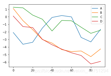
df = pd. DataFrame( np. random. randn( 10 , 4 ) . cumsum( 0 ) ,
index = np. arange( 0 , 100 , 10 ) ,
columns = [ 'A' , 'B' , 'C' , 'D' ] )
df. plot( )
df
A
B
C
D
0
-2.089443
1.089140
1.248430
0.082829
10
-3.649157
-0.520943
1.173340
-1.307401
20
-3.387452
-1.713291
0.212164
-1.434823
30
-1.511931
-3.020731
-0.334770
-2.991320
...
...
...
...
...
60
-0.027079
-4.617245
-0.540804
-4.774767
70
-2.743985
-4.534934
-1.393246
-5.132394
80
-3.336041
-5.283589
-2.202856
-6.250555
90
-1.680583
-4.269342
-1.783487
-5.914622
10 rows × 4 columns
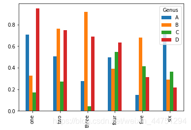
df = pd. DataFrame( np. random. rand( 6 , 4 ) ,
index = [ 'one' , 'two' , 'three' , 'four' , 'five' , 'six' ] ,
columns = pd. Index( [ 'A' , 'B' , 'C' , 'D' ] , name = 'Genus' ) )
df. plot( kind= 'bar' )
df
Genus
A
B
C
D
one
0.706566
0.326933
0.169319
0.950354
two
0.507864
0.763742
0.271822
0.750882
three
0.274819
0.916360
0.040567
0.688893
four
0.498586
0.390705
0.545891
0.636310
five
0.145746
0.681933
0.411809
0.314657
six
0.721254
0.289420
0.362825
0.218710
tips = pd. read_csv( './tips.csv' )
tips. total_bill. plot( kind= 'hist' , bins= 50 )
tips
total_bill
tip
sex
smoker
day
time
size
0
16.99
1.01
Female
No
Sun
Dinner
2
1
10.34
1.66
Male
No
Sun
Dinner
3
2
21.01
3.50
Male
No
Sun
Dinner
3
3
23.68
3.31
Male
No
Sun
Dinner
2
...
...
...
...
...
...
...
...
240
27.18
2.00
Female
Yes
Sat
Dinner
2
241
22.67
2.00
Male
Yes
Sat
Dinner
2
242
17.82
1.75
Male
No
Sat
Dinner
2
243
18.78
3.00
Female
No
Thur
Dinner
2
244 rows × 7 columns
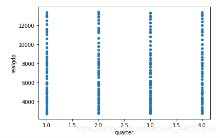
df = pd. read_csv( './macrodata.csv' )
data = df[ [ 'quarter' , 'realgdp' , 'realcons' ] ]
data. plot. scatter( 'quarter' , 'realgdp' )
data
quarter
realgdp
realcons
0
1.0
2710.349
1707.4
1
2.0
2778.801
1733.7
2
3.0
2775.488
1751.8
3
4.0
2785.204
1753.7
...
...
...
...
199
4.0
13141.920
9195.3
200
1.0
12925.410
9209.2
201
2.0
12901.504
9189.0
202
3.0
12990.341
9256.0
203 rows × 3 columns
gl = pd. read_csv( './game_logs.csv' )
gl. head( )
E:\anacanda\lib\site-packages\IPython\core\interactiveshell.py:3063: DtypeWarning: Columns (12,13,14,15,19,20,81,83,85,87,93,94,95,96,97,98,99,100,105,106,108,109,111,112,114,115,117,118,120,121,123,124,126,127,129,130,132,133,135,136,138,139,141,142,144,145,147,148,150,151,153,154,156,157,160) have mixed types.Specify dtype option on import or set low_memory=False.
  interactivity=interactivity, compiler=compiler, result=result)
date
number_of_game
day_of_week
v_name
v_league
v_game_number
h_name
h_league
h_game_number
v_score
...
h_player_7_name
h_player_7_def_pos
h_player_8_id
h_player_8_name
h_player_8_def_pos
h_player_9_id
h_player_9_name
h_player_9_def_pos
additional_info
acquisition_info
0
18710504
0
Thu
CL1
na
1
FW1
na
1
0
...
Ed Mincher
7.0
mcdej101
James McDermott
8.0
kellb105
Bill Kelly
9.0
NaN
Y
1
18710505
0
Fri
BS1
na
1
WS3
na
1
20
...
Asa Brainard
1.0
burrh101
Henry Burroughs
9.0
berth101
Henry Berthrong
8.0
HTBF
Y
2
18710506
0
Sat
CL1
na
2
RC1
na
1
12
...
Pony Sager
6.0
birdg101
George Bird
7.0
stirg101
Gat Stires
9.0
NaN
Y
3
18710508
0
Mon
CL1
na
3
CH1
na
1
12
...
Ed Duffy
6.0
pinke101
Ed Pinkham
5.0
zettg101
George Zettlein
1.0
NaN
Y
4
18710509
0
Tue
BS1
na
2
TRO
na
1
9
...
Steve Bellan
5.0
pikel101
Lip Pike
3.0
cravb101
Bill Craver
6.0
HTBF
Y
5 rows × 161 columns
gl. shape
(171907, 161)
gl. info( memory_usage= 'deep' )
<class 'pandas.core.frame.DataFrame'>
RangeIndex: 171907 entries, 0 to 171906
Columns: 161 entries, date to acquisition_info
dtypes: float64(77), int64(6), object(78)
memory usage: 860.5 MB
可以看见这份数据读取进来之后占用860.5MB内容
for dtype in [ 'float64' , 'object' , 'int64' ] :
selected_dtype = gl. select_dtypes( include= [ dtype] )
mean_usage_b = selected_dtype. memory_usage( deep= True ) . mean( )
mean_usage_mb = mean_usage_b / 1024 ** 2
print ( "Average memory usage for {} columns: {:03.2f} MB" . format ( dtype, mean_usage_mb) )
Average memory usage for float64 columns: 1.29 MB
Average memory usage for object columns: 9.51 MB
Average memory usage for int64 columns: 1.12 MB
循环中遍历3种类型,通过select_dtypes选中当前类型的特征,可以发现object类型占用的内存最多,其余int64和float64的两种差不多,我们需要对着三种数据类型进行处理,所得数据加载得考研快一点
首先,我们先了解一些数据的类型,int64,int32等类型
int_types = [ "uint8" , "int8" , "int16" , "int32" , "int64" ]
for it in int_types:
print ( np. iinfo( it) )
Machine parameters for uint8
---------------------------------------------------------------
min = 0
max = 255
---------------------------------------------------------------

Machine parameters for int8
---------------------------------------------------------------
min = -128
max = 127
---------------------------------------------------------------

Machine parameters for int16
---------------------------------------------------------------
min = -32768
max = 32767
---------------------------------------------------------------

Machine parameters for int32
---------------------------------------------------------------
min = -2147483648
max = 2147483647
---------------------------------------------------------------

Machine parameters for int64
---------------------------------------------------------------
min = -9223372036854775808
max = 9223372036854775807
---------------------------------------------------------------
def mem_usage ( pandas_obj) :
if isinstance ( pandas_obj, pd. DataFrame) :
usage_b = pandas_obj. memory_usage( deep= True ) . sum ( )
else :
usage_b = pandas_obj. memory_usage( deep= True )
usage_mb = usage_b / 1024 ** 2
return "{:03.2f} MB" . format ( usage_mb)
gl_int = gl. select_dtypes( include= [ 'int64' ] )
converted_int = gl_int. apply ( pd. to_numeric, downcast= 'unsigned' )
print ( mem_usage( gl_int) )
print ( mem_usage( converted_int) )
7.87 MB
1.48 MB
7.87 MB是全部为int64类型时的内存占用量
1.48 MB是向下转换后,int类型数据的内存占用量
mem_usage()函数的主要功能就是计算传入数据的内存占用量
gl_float = gl. select_dtypes( include= [ 'float64' ] )
converted_float = gl_float. apply ( pd. to_numeric, downcast= 'float' )
print ( mem_usage( gl_float) )
print ( mem_usage( converted_float) )
100.99 MB
50.49 MB
可以看见float类型向下转换基本上可以节省一半的内存
gl_obj = gl. select_dtypes( include= [ 'object' ] ) . copy( )
converted_obj = pd. DataFrame( )
for col in gl_obj. columns:
num_unique_values = len ( gl_obj[ col] . unique( ) )
num_total_values = len ( gl_obj[ col] )
if num_unique_values / num_total_values < 0.5 :
converted_obj. loc[ : , col] = gl_obj[ col] . astype( 'category' )
else :
converted_obj. loc[ : , col] = gl_obj[ col]
print ( mem_usage( gl_obj) )
print ( mem_usage( converted_obj) )
751.64 MB
51.67 MB
对object类型数据中唯一值个数进行判断,如果数量不足整体一半则进行转换,如果过多就忽略