Probabilistic Graphical Model (PGM) 概率图模型框架详解

往期文章链接目录

Probabilistic Graphical Model (PGM)

Definition: A probabilistic graphical model is a probabilistic model for which a graph expresses the conditional dependence structure between random variables.

In general, PGM obeys following rules:
$\begin{aligned} &\text {Sum Rule : } p\left(x_{1}\right)=\int p\left(x_{1}, x_{2}\right) d x_{2}\\ &\text {Product Rule : } p\left(x_{1}, x_{2}\right)=p\left(x_{1} | x_{2}\right) p\left(x_{2}\right)\\ &\text {Chain Rule: } p\left(x_{1}, x_{2}, \cdots, x_{p}\right)=\prod_{i=1}^{p} p\left(x_{i} | x_{i+1, x_{i+2}} \ldots x_{p}\right)\\ &\text {Bayesian Rule: } p\left(x_{1} | x_{2}\right)=\frac{p\left(x_{2} | x_{1}\right) p\left(x_{1}\right)}{p\left(x_{2}\right)} \end{aligned}$

As the dimension of the data increases, the chain rule is harder to compute. In fact, many models try to simplify it in some ways.

Why we need probabilistic graphical models

Reasons:

• They provide a simple way to visualize the structure of a probabilistic model and can be used to design and motivate new models.

• Insights into the properties of the model, including conditional independence properties, can be obtained by inspection of the graph.

• Complex computations, required to perform inference and learning in sophisticated models, can be expressed in terms of graphical manipulations, in which underlying mathematical expressions are carried along implicitly.

Three major parts of PGM

• Representation: Express a probability distribution that models some real-world phenomenon.

• Inference: Obtain answers to relevant questions from our models.

• Learning: Fit a model to real-world data.

We are going to mainly focus on Representation in this post.

Representation

Representation: Express a probability distribution that models some real-world phenomenon.

Directed graphical models (Bayesian networks)

Directed graphical models is also known as Bayesian networks.

Intuition:

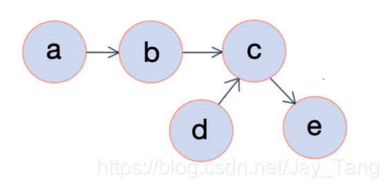
In a directed graph, vertices correspond to variables $x_i$ and edges indicate dependency relationships. Once the graphical representation of a directed graph is given (directed acyclic graphs), we can easily calculate the joint probability. For example, from the figure above, we can calculate the joint probability $p(a,b,c,d,e)$ by

$p(a,b,c,d,e) = p(a) \cdot p(b|a) \cdot p(c|b,d) \cdot p(d) \cdot p(e|c)$

Formal Definition:

A Bayesian network is a directed graph $G= (V,E)$ together with

• A random variable $x_i$ for each node $i \in V$.

• One conditional probability distribution (CPD) $p(x_i \mid x_{A_i})$ per node, specifying the probability of $x_i$ conditioned on its parents’ values.

Note:

• Bayesian networks represent probability distributions that can be formed via products of smaller, local conditional probability distributions (one for each variable). Another way to say it is that each factor in the factorization of $p(a,b,c,d,e)$ is locally normalized (every factor can sum up to one).

• Directed models are often used as generative models.

Undirected graphical models (Markov random fields)

Undirected graphical models is also known as Markov random fields (MRFs).

Unlike in the directed case, we cannot say anything about how one variable is generated from another set of variables (as a conditional probability distribution would do).

Intuition:

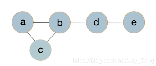
Suppose we have five students doing a project and we want to evaluate how well they would cooperate together. Since five people are too many to be evaluated as a whole, we devide it into small subgroups and evaluate these subgroups respectively. In fact, these small subgroups are called clique and we would introduce it later in this section.

Here, we introduce the concept of potential function $\phi$ to evaluete how well they would cooperate together. You can think of it as a score that measures how well a clique cooperate. Higher scores indicate better cooperation. In fact, we requie scores to be non-negative, and depending on how we define the potential functions, we would get different models. As the figure shown above, we could write $p(a,b,c,d,e)$ as

$p(a,b,c,d,e) = \phi_1(a,b,c) \cdot \phi_2(b,d) \cdot \phi_3(d,e)$

Note that the left hand side of the queation is a probability but the right hand side is a product of potentials/ scores. To make the right hand side a valid probability, we need to introduce a normalization term $1/Z$. Hence it becomes

$p(a,b,c,d,e) = \frac{1}{Z} \cdot \phi_1(a,b,c) \cdot \phi_2(b,d) \cdot \phi_3(d,e)$

Here we say $p(a,b,c,d,e)$ is globally normalized. Also, we call $Z$ a partition function, which is

$Z = \sum_{a,b,c,d,e} \phi_1(a,b,c) \cdot \phi_2(b,d) \cdot \phi_3(d,e) \tag 1$

Notice that the summation in $(1)$ is over the exponentially many possible assignments to $a,b,c,d$ and $e$. For this reason, computing $Z$ is intractable in general, but much work exists on how to approximate it.

Formal Definition:

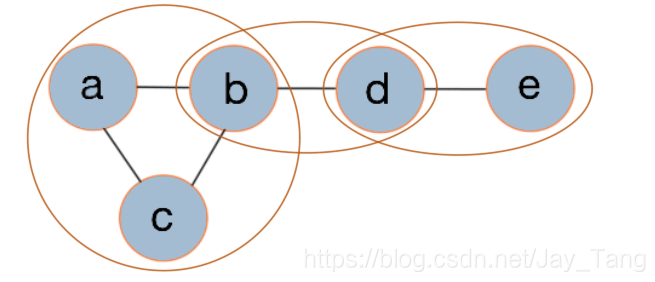
• cliques: fully connected subgraphs.

• maximal clique: A clique is a maximal clique if it is not contained in any larger clique.

A Markov Random Field (MRF) is a probability distribution $p$ over variables $x_{1}, \ldots, x_{n}$ defined by an undirected graph $G$ in which nodes correspond to variables $x_{i} .$ The probability $p$ has the form

$p\left(x_{1}, \ldots, x_{n}\right)=\frac{1}{Z} \prod_{c \in C} \phi_{c}\left(x_{c}\right) \tag 2$

where $C$ denotes the set of cliques of $G,$ and each factor $\phi_{c}$ is a non-negative function over the variables in a clique. The partition function

$Z=\sum_{x_{1}, \ldots, x_{n}} \prod_{c \in C} \phi_{c}\left(x_{c}\right)$

is a normalizing constant that ensures that the distribution sums to one.

Markov Properties of undirected graph

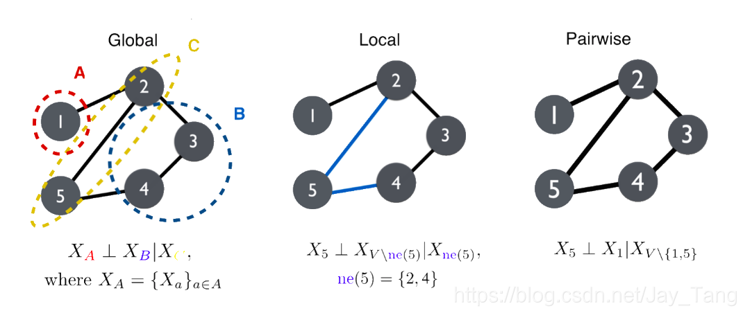
• Global Markov Property: $p$ satisfies the global Markov property with respect to a graph $G$ if for any disjoint vertex subsets $A$, $B$, and $C$, such that $C$ separates $A$ and $B$, the random variables $X_A$ are conditionally independent of $X_B$ given $X_C$.
  Here,we say $C$ separates $A$ and $B$ if every path from a node in $A$ to a node in B passes through a node in $C$ (d-seperation).

• Local Markov Property: $p$ satisfies the local Markov property with respect to $G$ if the conditional distribution of a variable given its neighbors is independent of the remaining nodes.

• Pairwise Markov Property: $p$ satisfies the pairwise markov property with respect to $G$ if for any pair of non-adjacent nodes, $s,t \in V$, we have $X_{s} \perp X_{t} | X_{V \backslash\{s, t\}}$.

Note:

• A distribution $p$ that satisfies the global Markov property is said to be a Markov random field or Markov network with respect to the graph.

• Global Markov Property $\Rightarrow$ Local Markov Property $\Rightarrow$Pairwise Markov Property.

• A Markov random field reflects conditional independency since it satisfies the Local Markov Property.

• To see whether a distribution is a Markov random field or Markov network, we have the following theorem:

  Hammersley-Clifford Theorem: Suppose $p$ is a strictly positive distribution, and $G$ is an undirected graph that indexes the domain of $p$. Then $p$ is Markov with respect to G if and only if $p$ factorizes over the cliques of the graph $G$.

Comparison between Bayesian networks and Markov random fields

• Bayesian networks effectively show causality, whereas MRFs cannot. Thus, MRFs are preferable for problems where there is no clear causality between random variables.

• It is much easier to generate data from a Bayesian network, which is important in some applications.

• In Markov random fields, computing the normalization constant $Z$ requires a summation over the exponentially many possible assignments. For this reason, computing $Z$ is intractable in general, but much work exists on how to approximate it.

Moral graph

A moral graph is used to find the equivalent undirected form of a directed acyclic graph.

The moralized counterpart of a directed acyclic graph is formed by

1. Add edges between all pairs of non-adjacent nodes that have a common child.

2. Make all edges in the graph undirected.

Here is an example:

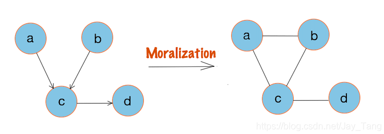
Note that a Bayesian network can always be converted into an undirected network.

Therefore, MRFs have more power than Bayesian networks, but are more difficult to deal with computationally. A general rule of thumb is to use Bayesian networks whenever possible, and only switch to MRFs if there is no natural way to model the problem with a directed graph

Factor Graph

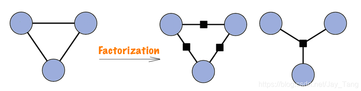
A Markov network has an undesirable ambiguity from the factorization perspective. Consider the three-node Markov network in the figure (left). Any distribution that factorizes as

$p(x_1, x_2, x_3) \propto \phi(x_1,x_2,x_3) \tag 3$

for some positive function $\phi$ is Markov with respect to this graph (check Hammersley-Clifford Theorem mentioned earlier). However, we may wish to use a more restricted parameterization, where

$p(x1, x2, x3) \propto \phi_1(x_1, x_2)\phi_1(x_2, x_3)\phi_1(x_1, x_3) \tag 4$

The model family in $(4)$ is smaller, and therefore may be more amenable to parameter estimation. But the Markov network formalism cannot distinguish between these two parameterizations. In order to state models more precisely, the factorization in $(2)$ can be represented directly by means of a factor graph.

Definition (factor graph): A factor graph is a bipartite graph $G = (V, F, E)$ in which a variable node $x_i \in V$ is connected to a factor node $\phi_a \in F$ if $x_i$ is an argument to $\phi_a$.

An example of a factor graph is shown on the right side of the figure above. In the figure, the circles are variable nodes, and the shaded boxes are factor nodes. Notice that, unlike the undirected graph, the factor graph depicts the factorization of the model unambiguously.

Remark: Directed models can be thought of as a kind of factor graph, in which the individual factors are locally normalized in a special fashion so that globally $Z = 1$.

Inference

Inference: Obtain answers to relevant questions from our models.

• Marginal inference: what is the probability of a given variable in our model after we sum everything else out?

$p(y=1) = \sum_{x_1} \sum_{x_2} \cdots \sum_{x_n} p(y=1, x_1, x_2, \dotsc, x_n)$

• Maximum a posteriori (MAP) inference: what is the most likely assignment to the variables in the model?

$\max_{x_1, \dotsc, x_n} p(y=1, x_1, \dotsc, x_n)$

Learning

Learning: Fit a model to real-world data.

• Parameter learning: the graph structure is known and we want to estimate the parameters.

  • complete case:

    • We use Maximum Likelihood Estimation to estimate parameters.

  • incomplete case:

    • We use EM Algorithm to approximate parameters.

    • Example: Guassian Mixture Model (GMM), Hidden Markov Model (HMM).

• Structure learning: we want to estimate the graph, i.e., determine from data how the variables depend on each other.

---

Reference:

• Bishop, Christopher M., “Pattern Recognition and Machine Learning,” Springer, 2006.
• https://ermongroup.github.io/cs228-notes/
• https://en.wikipedia.org/wiki/Moral_graph
• https://space.bilibili.com/97068901
• https://zhenkewu.com/assets/pdfs/slides/teaching/2016/biostat830/lecture_notes/Lecture4.pdf
• https://skggm.github.io/skggm/tour
• https://homepages.inf.ed.ac.uk/csutton/publications/crftutv2.pdf

往期文章链接目录