What is mode collapse?
Most interesting real-world data distributions are highly complex and multimodal. That is to say, the probability distribution which describes the data has multiple “peaks” where different sub-groups of samples are concentrated.
For example, let’s say you have a dataset containing a mixture of summer day temperature readings from Alice Springs in central Australia (typically very hot) and the South Pole in Antarctica (typically very cold). The distribution of the data is bimodal - there are peaks at the average temperatures of the two places with a gap inbetween. The graph below illustrates this more clearly.
Now let’s say you want to train a GAN which produces plausible temperature values. Intuitively speaking, we would expect the generator to learn to produce hot and cold temperatures with roughly equal probability. However, a commonly encountered issue is that a mode collapse will occur, resulting in the generator only outputting samples from a single mode (eg only cold temperatures). To understand why, consider the following scenario:
The generator learns that it can fool the discriminator into thinking that it is outputting realistic temperatures by producing values close to Antarctic temperatures.
The discriminator counters by learning that all Australian temperatures are real (not produced by the generator), and essentially guesses whether Antarctic temperatures are real or fake since they are indistinguishable.
The generator exploits the discriminator by switching modes to produce values close to Australian temperatures instead, abandoning the Antarctic mode.
The discriminator now assumes that all Australian temperatures are fake and Antarctic temperatures are real.
Return to step 1.
This game of cat-and-mouse repeats ad nauseum, with the generator never being directly incentivised to cover both modes. In such a scenario the generator will exhibit very poor diversity amongst generated samples, which limits the usefulness of the learnt GAN.
In reality, the severity of mode collapse varies from complete collapse (all generated samples are virtually identical) to partial collapse (most of the samples share some common properties). Unfortunately, mode collapse can be triggered in a seemingly random fashion, making it very difficult to play around with GAN architectures.
Addressing mode collapse
Mode collapse is a well-recognised problem, and researchers have made a few attempts at addressing it. I have identified 4 broad approaches to tackling mode collapse, which are described below.
Directly encourage diversity
It is impossible to determine output diversity by considering individual samples in isolation. This leads to a very logical next step of using batches of samples to directly assess diversity. Minibatch discrimination and feature mapping 1 are two techniques which fall into this category.
Minibatch discrimination gives the discriminator the power of comparing samples across a batch to help determine whether the batch is real or fake.
Feature matching modifies the generator cost function to factor in the diversity of generated batches. It does this by matching statistics of discriminator features for fake batches to those of real batches. I had some success combining feature matching with the traditional GAN generator loss function to form a hybrid objective.
Anticipate counterplay
One way to prevent the cat-and-mouse game of hopping between modes is to peek into the future and anticipate counterplay when updating parameters. This approach should be familiar to those who know a bit about game theory (eg minimax). Intuitively, this prevents players of the GAN game from making moves which are easily countered.
Unrolled GANs 2 take this kind of approach by allowing the generator to “unroll” updates of the discriminator in a fully differentiable way. Now instead of the generator learning to fool the current discriminator, it learns to maximally fool the discriminator after it has a chance to respond, thus taking counterplay into account. Downsides of this approach are increased training time (each generator update has to simulate multiple discriminator updates) and a more complicated gradient calculation (backprop through an optimiser update step can be difficult).
Use experience replay
Hopping back and forth between modes can be minimised by showing old fake samples to the discriminator every so often. This prevents the discriminator from becoming too exploitable, but only for modes that have already been explored by the generator in the past.
A similar kind of effect can be achieved by occasionally substituting in an old discriminator/generator for a few iterations.
Use multiple GANs
Rather than fight mode collapse we could simply accept that the GAN will cover only a subset of the modes in the dataset, and train multiple GANs for different modes. When combined, these GANs cover all of the modes. AdaGAN 3 takes this approach. The major downside here is that training multiple GANs takes a lot of time. Furthermore, using a combination of GANs is generally more unwieldy than working with just one.
How about tweaking the objective?
In an earlier post I took a look at the GAN objective function and mentioned that different f-divergences have different mode-seeking vs mode-covering behaviour. It is my current belief that this has minimal (if any) impact on the mode collapse problem described here. No matter what the objective function is, if it only considers individual samples (without looking forward or backward) then the generator is not directly incentivised to produce diverse examples.
Section 3.2.5 of “NIPS 2016 Tutorial: Generative Adversarial Networks” 4 covers this point in more detail.
References
Improved Techniques for Training GANs. https://arxiv.org/abs/1606.03498
Unrolled Generative Adversarial Networks. https://arxiv.org/abs/1611.02163
AdaGAN: Boosting Generative Models. https://arxiv.org/abs/1701.02386v1
NIPS 2016 Tutorial: Generative Adversarial Networks.
https://arxiv.org/abs/1701.00160v3
---------------------
作者:witnessai1
来源:CSDN
原文:https://blog.csdn.net/witnessai1/article/details/79493181
版权声明:本文为博主原创文章,转载请附上博文链接!
解决模式崩溃
模式崩溃是一个公认的问题,研究人员已经做了一些尝试来解决它。我已经确定了4种处理模式崩溃的方法,如下所述。
直接鼓励多样性
单独考虑单个样本是不可能确定输出多样性的。这就引出了一个非常合乎逻辑的下一步,即使用批量样本直接评估多样性。小批量识别和特征映射是属于这一类的两种技术。小批量鉴别赋予鉴别器跨批比较样本的能力,以帮助确定批是真还是假。
特征匹配修改了生成器的成本函数,以将生成的批的多样性考虑在内。它通过匹配鉴别器特征的统计信息来实现这一点
预计反攻
防止模式间跳来跳去的猫鼠游戏的一种方法是预测未来,并在更新参数时预测对策。这种方法对于那些稍微了解博弈论(如极小极大)的人应该很熟悉。直观地说,这阻止了GAN游戏的玩家做出容易被反击的动作。
展开的GANs 2采用这种方法,允许生成器以完全可微的方式“展开”鉴别器的更新。现在不是生成器学习欺骗当前的鉴别器,而是学习最大限度地欺骗t
使用经验重播
通过每隔一段时间向鉴别器显示旧的假样本,可以使模式间的跳来跳去最小化。这可以防止鉴别器变得太容易被利用,但仅限于生成器过去已经探索过的模式。
类似的效果可以通过偶尔用一个旧的鉴别器/生成器替换几个迭代来实现。
使用多个GAN
我们可以简单地接受GAN只覆盖数据集中模式的一个子集,并为不同模式训练多个GANs,而不是对抗模式崩溃。当合并时,这些GANs覆盖所有模式。AdaGAN 3采用了这种方法。这里的主要缺点是训练多个GANs需要很多时间。此外,使用甘斯的组合通常比只使用一个甘斯更笨拙。
调整一下目标如何?
在之前的一篇文章中,我研究了GAN目标函数,并提到不同的f-分歧具有不同的模式寻求和模式覆盖行为。我目前认为,这对这里描述的模式崩溃问题影响很小(如果有的话)。无论目标函数是什么,如果它只考虑单个样本(不向前看或向后看),那么生成器就不会直接受到激励来生成不同的示例。
对抗生成网络被广泛应用于图像生成领域,比较常用的有超分辨率,图像翻译,卡通人物生成,人体姿态生成,年龄变换,风格变换等等,超乎想象,精彩纷呈。另一方面,GAN模型训练困难,变化无常,神秘莫测。由于其强烈的不稳定性,目前难以大规模实用。
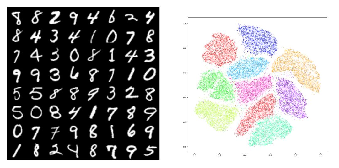
图1. MNIST数据集 tSNE 嵌入在平面上,10个团簇对应着10个模式(modes)。模式崩溃(Mode Collapse)指生成模型只生成其中的几种模式。
如图1所示,给定数据集合,我们用编码映射将其映入隐空间中,每个数字对应一个团簇,即MNIST数据的概率分布密度函数具有多个峰值,每个峰值被称为是一个模式(mode)。理想情况下,生成模型应该能够生成10个数字,如果只能生成其中的几个,而错失其它的模式,则我们称这种现象为模式崩溃(mode collapse)。
具体而言,GAN训练中经常出现如下三个层次的问题:
我们将这些现象笼统称为广义的模式崩溃问题。如何解释模式崩溃的原因,如何设计新型算法避免模式崩溃,这些是深度学习领域的最为基本的问题。我们用最优传输中的Brenier理论,和蒙日-安培方程(Monge-Ampere)的正则性(regularity)理论来解释模式崩溃问题。
GAN和蒙日-安培方程
我们以前讨论过对抗生成网络的:生成器(Generator)将隐空间的高斯分布变换成数据流形上一个分布,判别器(Discriminator)计算生成分布和真实数据分布之间的距离,例如Wasserstein距离。这些操作本质上都可以用,并且加以改进。以欧氏距离平方为代价函数的最优传输问题归结为Brenier理论,并且等价于凸几何中的Alexandrov理论,最终归结为蒙日-安培方程。
假设在隐空间中,在源区域上定义了概率测度,在目标区域上定义了概率测度,,。同时存在,满足,由Brenier定理,存在全局Lipschitz凸函数,其梯度映射给出最优传输映射,即保持测度:对于任意Borel集合,,
同时极小化传输代价
这里凸函数被称为是Brenier势能函数。Brenier势能函数给出蒙日-安培方程(Monge-Ampere Equation)的弱解:
在工程计算中,我们通常用Alexandrov弱解来逼近真实解,我们以前讨论过Alexandrov弱解的存在性和唯一性。
蒙日-安培方程的正则性理论
Brenier势能函数是蒙日-安培方程的解,其光滑性是一个错综复杂的问题。汪徐家教授是这一领域的国际权威之一,给了老顾很多帮助。我们假设源域是凸区域,如果也是凸区域,那么Caffarelli理论给出了Brenier势能函数的正则性。我们回忆赫德尔系数(Holder coefficient)为
赫德尔空间定义为:
如果密度函数,,那么Brenier势能函数,这里并且。
但是,如果目标概率分布的支集非凸,那么即便密度函数光滑,蒙日-安培方程的解有可能不可微,,进一步最优传输映射非连续。
由Brenier定理,Brenier势能函数为整体Lipschitz,因此几乎处处可导。我们称可求导的点为正常点(regular point),不可求导的点为奇异点(singular point),则奇异点集合为零测度。我们考察每一点处的次微分,
定义(次微分)一个凸函数在点的次微分(subdifferential)定义为集合
正常点的次微分只包含函数的梯度,即 ,奇异点的次微分是一个无穷集合。我们定义集合,
显然,是正常点集合,是奇异点集合,这里。每一个奇异点都可以用正常点的Cauchy序列来逼近,由此,我们可以定义可达次微分,
可以证明:次微分等于可达次微分的凸包(convex hull),
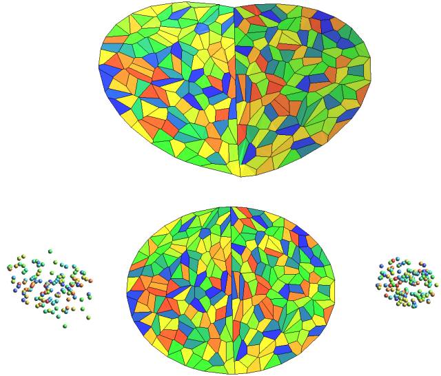
图2. 最优传输映射中的奇异点集合,(苏科华作)。
如图2所示,目标测度的支集具有两个联通分支,我们稠密采样目标测度,表示成定义在两个团簇上面的狄拉克测度。我们然后计算蒙日-安培方程的Alenxandrov解。依随采样密度增加,狄拉克测度弱收敛到目标测度,Alenxandrov解收敛到真实解。我们看到Brenier势能函数的Alenxandrov解可以表示成一张凸曲面,图曲面中间有一条脊线(ridge),脊线的投影是最优传输映射的奇异点集。
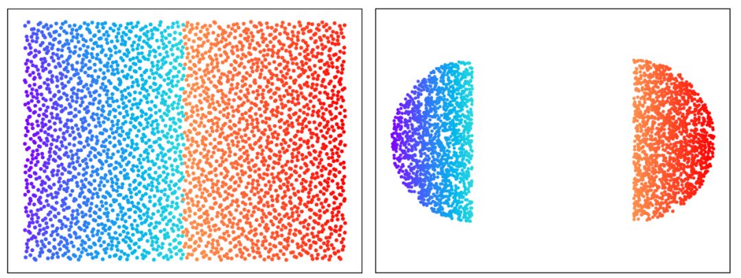
图3. GPU版本的最优传输映射(郭洋、Simon Lam 作)。
图3显示了基于GPU算法的从平面长方形上的均匀分布到两个半圆盘上的均匀分布的最优传输映射,长方形的中线显示了最优传输映射的奇异点集。
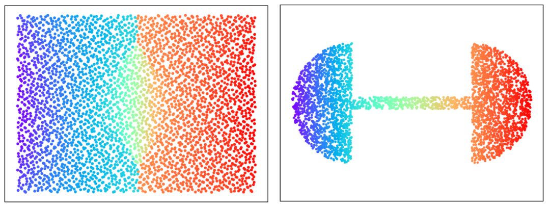
图4. GPU版本的最优传输映射(郭洋、Simon Lam作)。
图4从平面长方形上的均匀分布到哑铃形状上的均匀分布的最优传输映射,仔细观察,我们可以看出最优传输映射的奇异点集是中线上的两条线段,介于红蓝斑点之间。
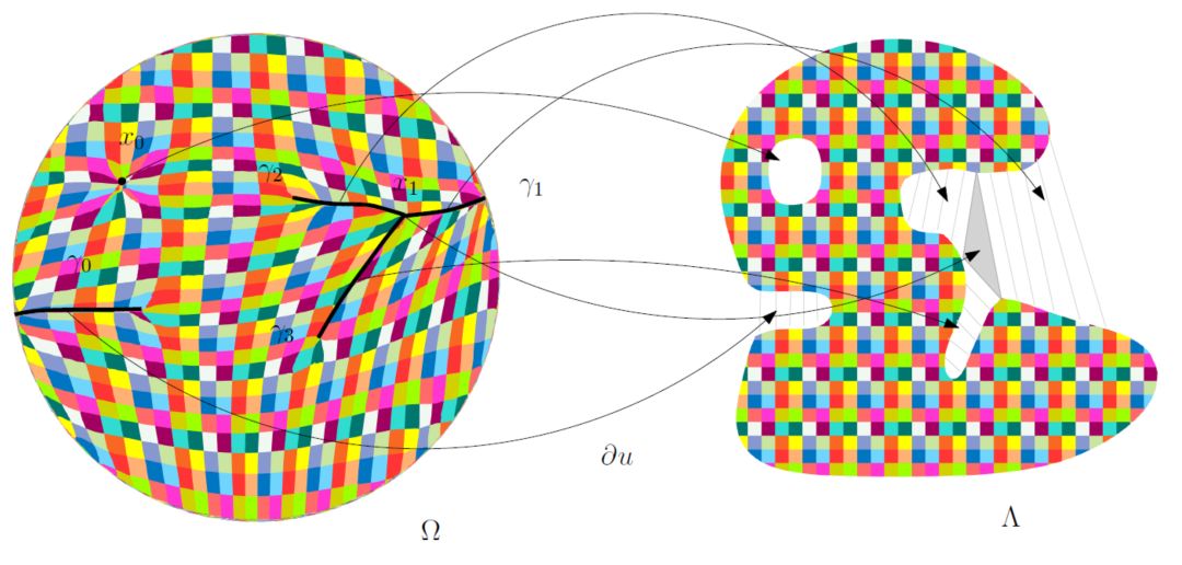
图5. 最优传输映射的奇异点结构(齐鑫、苏科华作)。
图5显示了二维最优传输映射的奇异点结构:这里源区域是单位圆盘,目标区域是平面上非凸区域,带有一个孔洞。Breinier势能函数的奇异点集标注在左帧,,每个奇异点的次微分覆盖一个二维区域,覆盖的孔洞,覆盖右侧的灰色三角形;
每一条曲线覆盖边界处的一个“豁口”,上的任意一点,次微分是外、联结着边界上两点的直线段,可达次微分是边界上的那两点。奇异点的测度为0,Brenier势能函数几乎处处可微,最优传输映射在上几乎处处连续,在上间断。
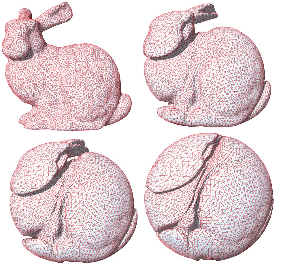
图6. 实心兔子和实心球之间的最优传输映射,表面皱褶结构,(苏科华作)。
最优传输映射的奇异点结构理论在高维空间依然成立,如图6所示,实心球体和实心兔子体之间的最优传输映射诱导了兔子表面上的大量皱褶,最优传输映射在皱褶处间断。
最优传输映射具有奇异点,那么一般传输映射又会如何?假设我们有映射,将概率测度推前到概率测度,Brenier极分解定理断言,存在唯一的分解, 这里是最优传输映射,是雅可比行列式处处为1的自映射。由此,一般的传输映射也存在奇异点,映射在奇异点处间断。
模式崩溃的理论解释
目前的深度神经网络只能够逼近连续映射,而传输映射是具有间断点的非连续映射,换言之,GAN训练过程中,目标映射不在DNN的可表示泛函空间之中,这一显而易见的矛盾导致了收敛困难;如果目标概率测度的支集具有多个联通分支,GAN训练得到的又是连续映射,则有可能连续映射的值域集中在某一个连通分支上,这就是模式崩溃(mode collapse);如果强行用一个连续映射来覆盖所有的连通分支,那么这一连续映射的值域必然会覆盖之外的一些区域,即GAN会生成一些没有现实意义的图片。这给出了GAN模式崩溃的直接解释。
那么,如何来用真实数据验证我们的猜测呢?我们用CelebA数据集验证了传输映射的非连续性。
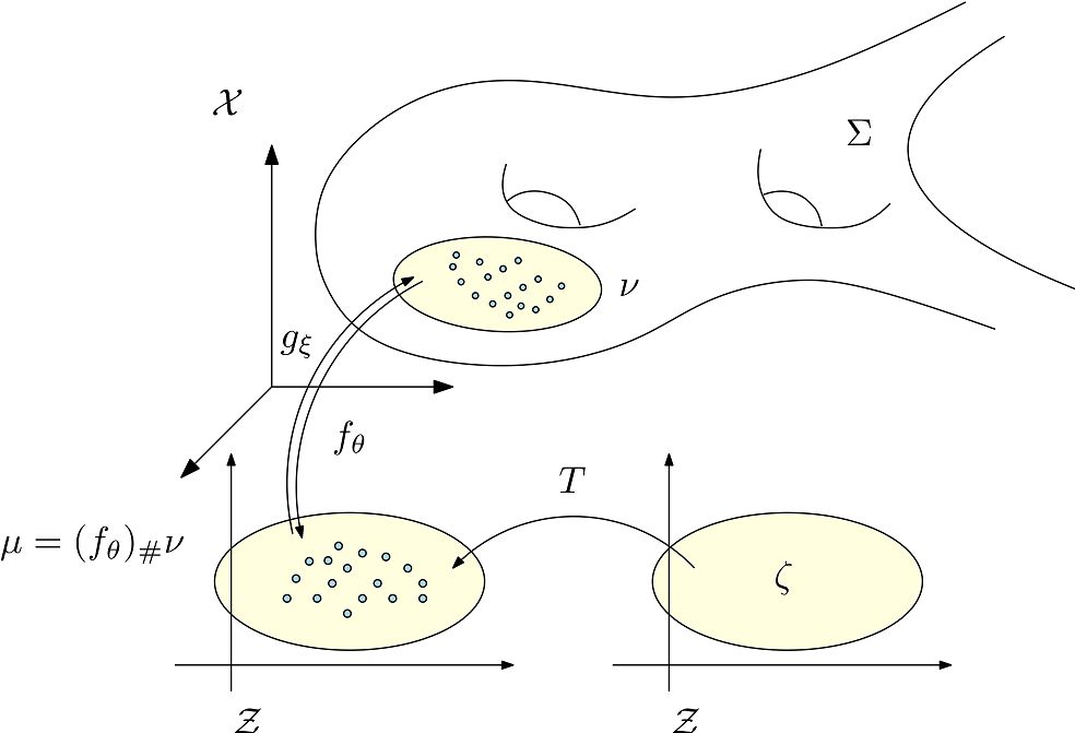
图7. AE-OT体系结构。
如图7所示我们认为人脸图片在图像空间中的分布集中在某个低维流形附近,我们用自动编码器(Autoencoder),将流形映入到隐空间中,编码映射记为,解码映射记为。编码映射将分布推前到隐空间的分布,的支集为。商空间中的最优传输映射为,这里是单位立方体,为均匀分布。我们在中随机采样,那么是生成的人脸图片。
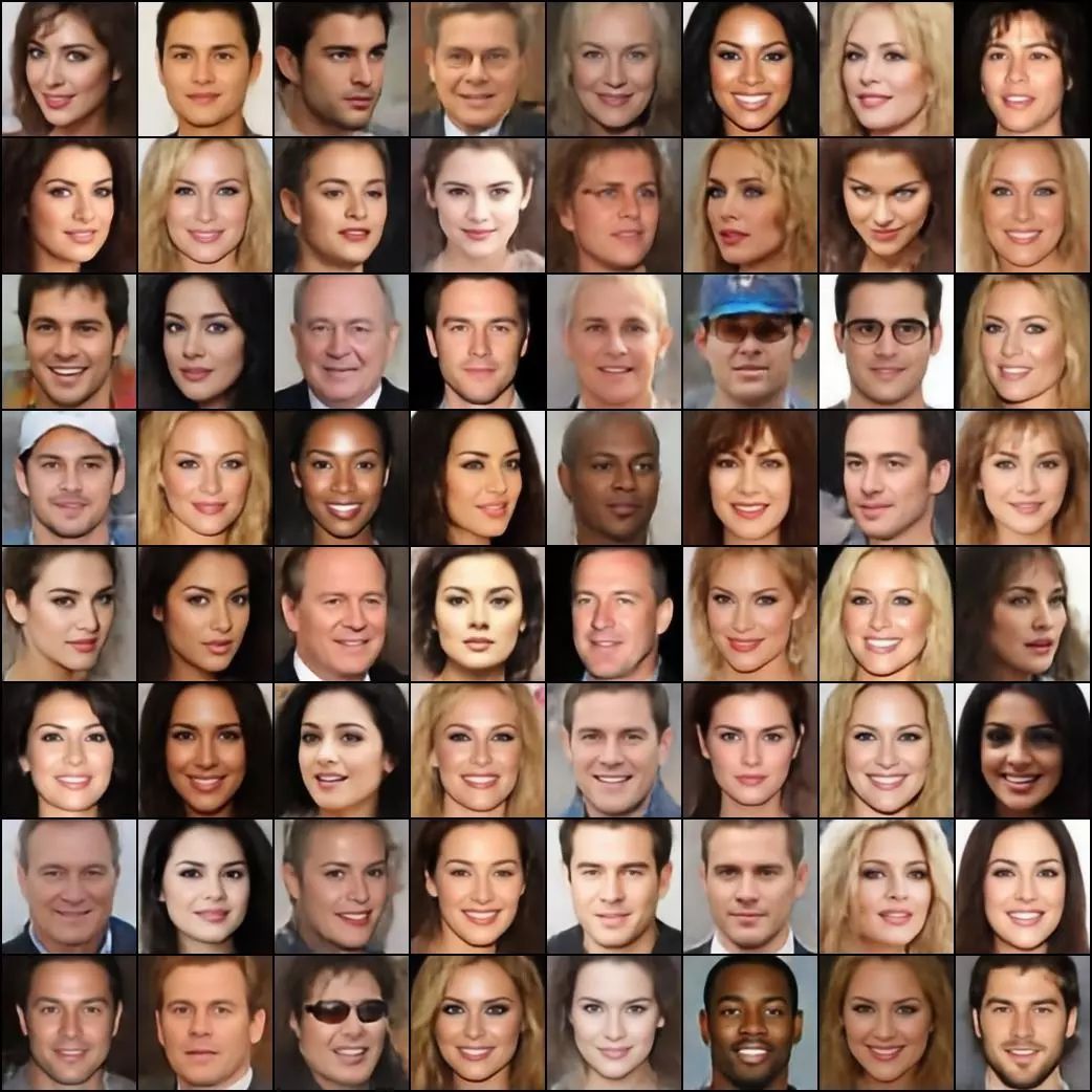
图8. AE-OT生成的人脸图像。
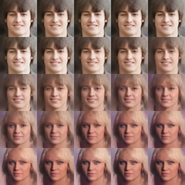
图10. 在隐空间进行插值的结果。
如图10所示,我们在隐空间中任选两点,然后画一条直线段,那么给出了一系列人脸图像,即人脸图像流形上的一条曲线。如果最优传输映射非连续,有可能和奇异点集相交,即直线段和某个皱褶相交,不妨设交点为,那么在人脸图像流形之外,即是一幅真实生活中不可能出现的人脸。图10中心显示了一幅人脸图像,左眼为棕色,右眼为蓝色,这是现实世界中几乎不可能的人脸。这意味着和奇异点集相交,传输映射非连续,存在间断点。
那么如何避免模式崩溃呢?通过以上分析我们知道,深度神经网络只能逼近连续映射,传输映射本身是非连续的,这一内在矛盾引发了模式崩溃。但是最优传输映射是Brenier势能函数的梯度,Brenier势能函数本身是连续的,因此深度神经网络应该来逼近Brenier势能函数,而非传输映射。更进一步,我们应该判断Brenier势能函数的奇异点,即图2中的脊线和图6中的皱褶。
小结
基于真实数据的流形分布假设,我们将深度学习的主要任务分解为学习流形结构和概率变换两部分;概率变换可以用最优传输理论来解释和实现。基于Brenier理论,我们发现GAN模型中的生成器D和判别器G计算的函数彼此可以相互表示,因此生成器和判别器应该交流中间计算结果,用合作代替竞争。Brenier理论等价于蒙日-安培方程,蒙日-安培方程正则性理论表明:如果目标概率分布的支集非凸,那么存在零测度的奇异点集,传输映射在奇异点处间断。而传统深度神经网络只能逼近连续映射,这一矛盾造成了模式崩溃。
通过计算Brenier势能函数,并且判定奇异点集,我们可以避免模式崩溃。这些算法存在GPU实现方式。这种方法更为稳定,鲁棒,训练效率大为提升,并且用透明的理论模型部分取代了经验的黑箱。
References
1. Na Lei, Yang Guo, Dongsheng An, Xin Qi, Zhongxuan Luo, Shing-Tung Yau, Xianfeng Gu. "Mode Collapse and Regularity of Optimal Transportation Maps", ArXiv:1902.02934返回搜狐,查看更多