【Python for Data Analysis】Numpy入门教程

4.1 NumPy ndarray

NumPy, short for Numerical Python, is the fundamental package required for high performance scientific computing and data analysis.

One of the key features of NumPy is its N-dimensional array object, or ndarray, which
is a fast, flexible container for large data sets in Python.

Whenever we see “array”, “Numpy array”, or “ndarray” in this book, with few exceptions they all refer to the same thing: the ndarray object

A ndarray example

array([[7, 5],
       [2, 3]])

---

import numpy as np
my_arr = np.arange(1000000)
my_list = list(range(1000000))

Run time

%time my_arr2 = my_arr * 2
%time my_list = my_list * 2

CPU times: user 3.99 ms, sys: 5.66 ms, total: 9.64 ms
Wall time: 13.1 ms
CPU times: user 20.3 ms, sys: 9.21 ms, total: 29.5 ms
Wall time: 39.1 ms

As we can see Numpy method is much faster than Python method, and cost less space.

4.1.1 Create ndarray

The easiest way to create an array is to use the array function

# data1 is a list
data1 = [[1, 2, 3], [4, 5, 6]]
array1 = np.array(data1)
array1
array1.shape

(2, 3)

data2 = [5, 4.1, 2, 8]
array2 = np.array(data2)
print(array2)
print(array2.dtype)

[5.  4.1 2.  8. ]
float64

print(np.zeros(4))

[0. 0. 0. 0.]

To create a higher dimensional array with these methods, pass a tuple for the shape

np.zeros((2,5)) # parameter Shape: int or tuple int

array([[0., 0., 0., 0., 0.],
       [0., 0., 0., 0., 0.]])

np.ones((3,4))

array([[1., 1., 1., 1.],
       [1., 1., 1., 1.],
       [1., 1., 1., 1.]])

empty creates an array without initializing its values to any particular value:

np.empty((1,2,3))

array([[[1.28822975e-231, 1.28822975e-231, 1.97626258e-323],
        [0.00000000e+000, 0.00000000e+000, 0.00000000e+000]]])

arange is an array-valued version of the built-in Python range function:

np.arange(1, 10, 2)

array([1, 3, 5, 7, 9])

list(range(1, 10, 2)) # function range return an iterable object, not a list

[1, 3, 5, 7, 9]

ones_like takes another array and produces a ones array of the same shape and dtype

np.ones_like([2,3,4]) 

array([1, 1, 1])

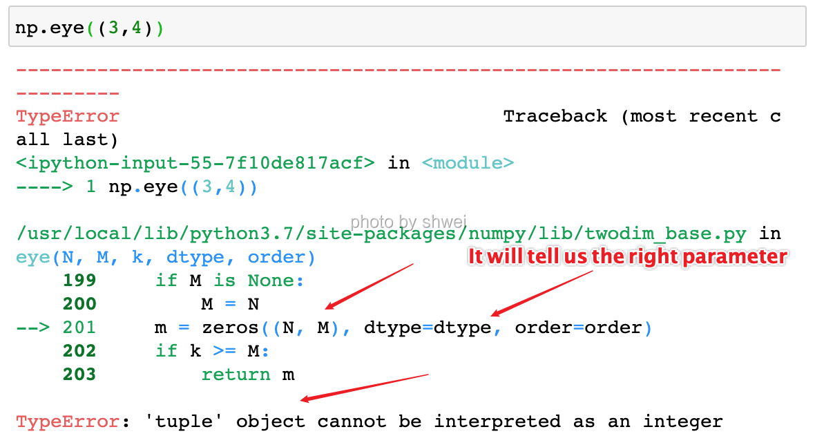
It will tell us the right parameters format, so we don’t need to memory them.

Create a square N * N identity matrix (1’s on the digonal and 0’s elsewhere)

np.identity(4)

array([[1., 0., 0., 0.],
       [0., 1., 0., 0.],
       [0., 0., 1., 0.],
       [0., 0., 0., 1.]])

np.eye(3,4)

array([[1., 0., 0., 0.],
       [0., 1., 0., 0.],
       [0., 0., 1., 0.]])

np.full([2,3], 5)

array([[5, 5, 5],
       [5, 5, 5]])

Table 4-1. Array creation functions

Function	Description
array	Convert input data (list, tuple, array, or other sequence type) to an ndarray either by inferring a dtype or explicitly specifying a dtype. Copies the input data by default.
asarray	Convert input to ndarray, but do not copy if the input is already an ndarray
arange	Like the built-in range but returns an ndarray instead of a list.
ones, ones_like	Produce an array of all 1’s with the given shape and dtype. ones_like takes another array and produces a ones array of the same shape and dtype.
zeros, zeros_like	Like ones and ones_like but producing arrays of 0’s instead
empty, empty_like	Create new arrays by allocating new memory, but do not populate with any values like ones and zeros
eye, identity	Create a square N x N identity matrix (1’s on the diagonal and 0’s elsewhere)

4.1.2 Data Types for ndarrays

The data type or dtype is a special object containing the information the ndarray needs to interpret a chunk of memory as a particular type of data:

The default dtype is float64

arr1 = np.array([1,2,3], dtype=np.float64)
arr2 = np.array([1,2,3.1], dtype=np.int32)
arr3 = np.ones(4) # use default dtype

arr1.dtype

dtype('float64')

arr1

array([1., 2., 3.])

arr2.dtype

dtype('int32')

arr2

array([1, 2, 3], dtype=int32)

arr3.dtype

dtype('float64')

arr3

array([1., 1., 1., 1.])

Table 4-2. NumPy data types

Type	Type Code	Description
int8, uint8	i1, u1	Signed and unsigned 8-bit (1 byte) integer types
int16, uint16	i2, u2	Signed and unsigned 16-bit integer types
int32, uint32	i4, u4	Signed and unsigned 32-bit integer types
int64, uint64	i8, u8 S	igned and unsigned 32-bit integer types
float16	f2	Half-precision floating point
float32	f4 or f	Standard single-precision floating point. Compatible with C float
float64, float128	f8 or d	Standard double-precision floating point. Compatible with C double and Python float object
float128	f16 or g	Extended-precision floating point
complex64, complex128, complex256	c8, c16, c32	Complex numbers represented by two 32, 64, or 128 floats, respectively
bool	?	Boolean type storing True and False values
object	O	Python object type
string_	S	Fixed-length string type (1 byte per character) . For example, to create a string dtype with length 10, use ‘S10’.
unicode_	U	Fixed-length unicode type (number of bytes platform specific). Same specification semantics as string_ (e.g. ‘U10’).

4.1.3 Operations between Arrays and Scalars

Arrays are important because they enable you to express batch operations on data without any for loops. This is usually called vectorization.

arr = np.array([[1,2,3],[4.,5,6]])

arr

array([[1., 2., 3.],
       [4., 5., 6.]])

arr * arr

array([[ 1.,  4.,  9.],
       [16., 25., 36.]])

1 / arr

array([[1.        , 0.5       , 0.33333333],
       [0.25      , 0.2       , 0.16666667]])

arr ** 0.5

array([[1.        , 1.41421356, 1.73205081],
       [2.        , 2.23606798, 2.44948974]])

arr2 = np.array([[0., 4., 1.], [7, 2,12.]])

arr2

array([[ 0.,  4.,  1.],
       [ 7.,  2., 12.]])

Comparing between two arrays of the same size return bool array

arr2 > arr

array([[False,  True, False],
       [ True, False,  True]])

Operations between differently sized arrays is called broadcasting. Having a deep understanding of broadcasting is not neccessay for most of this book.

4.1.4 Basic Indexing and Slicing

An important first distinction frome lists is that array slice are views on the original array. This means that the data is not copied, and any motifications to the view will be reflected in the source array.

arr = np.arange(10)

arr

array([0, 1, 2, 3, 4, 5, 6, 7, 8, 9])

# any motifications to the view will be reflected in the source array:
arr[5:8] = 12 

arr 

array([ 0,  1,  2,  3,  4, 12, 12, 12,  8,  9])

# array slice is not copied
arr_slice = arr[5:8]
arr_slice[1] = 100
arr

array([  0,   1,   2,   3,   4,  12, 100,  12,   8,   9])

# list slice is copied
list_ = list(range(10))
list_slice = list_[5:8]
list_slice[1] = 100

list_

[0, 1, 2, 3, 4, 5, 6, 7, 8, 9]

Notes: As Numpy has been designed with large data use cases in mind, you could imagine performance and memory problems if Numpy insisted on copying data left and right.

# array slice is copied if you use copy()
arr_slice = arr[5:8].copy()
arr_slice[1] = 888
arr

array([  0,   1,   2,   3,   4,  12, 100,  12,   8,   9])

higher dimensional array index

arr2d = np.array([[1,2],[3,4]])
arr2d[0]

array([1, 2])

You can pass a comma-separated list of indices to select individual elements.

So these are equivalent:

arr2d[0][1]

2

arr2d[0,1]

2

Note: they are different if it is a slice

4.1.4.1 Note the function of arr3d[ :2, 1:, 0]

use comma , to process each dimension

arr2d[:2,:1] # process each dimension

array([[1],
       [3]])

arr2d[:2][:1] 
# equivalent: tmp = arr2d[:2] and tmp[:1]

array([[1, 2]])

3D array

arr3d = np.array([ [[1,2,3], [4,5,6]],  
                  [[7,8,9], [10,11,12]]
                 ])
arr3d

array([[[ 1,  2,  3],
        [ 4,  5,  6]],

       [[ 7,  8,  9],
        [10, 11, 12]]])

integer indexes return lower dimensonal axes

arr3d[0] 

array([[1, 2, 3],
       [4, 5, 6]])

colon: return the same dimensional axes

arr3d[:1] 

array([[[1, 2, 3],
        [4, 5, 6]]])

arr3d[0,1]

array([4, 5, 6])

arr3d[0,1] = 0

arr3d

array([[[ 1,  2,  3],
        [ 0,  0,  0]],

       [[ 7,  8,  9],
        [10, 11, 12]]])

Note that in all of these cases where subsections of the array have been selected, the returned arrays are views, not copied.

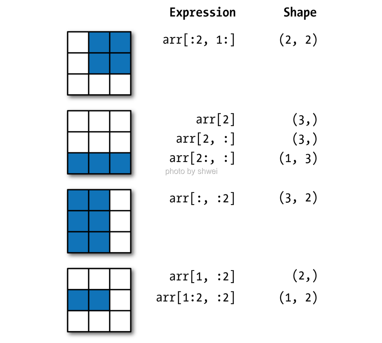
Indexing with slices

arr2d = np.array([[1,2,3],
                  [4,5,6],
                  [7,8,9]
                 ])

arr2d

array([[1, 2, 3],
       [4, 5, 6],
       [7, 8, 9]])

arr2d.shape

(3, 3)

arr2d[:1] # same dimensionality

array([[1, 2, 3]])

arr2d[0] # lower dimensionality

array([1, 2, 3])

arr2d[1,:2]

array([4, 5])

arr2d[:, :1]

array([[1],
       [4],
       [7]])

arr2d[:2, 1:]

array([[2, 3],
       [5, 6]])

arr2d[:2][1:]

array([[4, 5, 6]])

arr_test = arr2d[:2, 1:]
arr_test = 0

arr2d

array([[1, 2, 3],
       [4, 5, 6],
       [7, 8, 9]])

arr2d[:2, 1:] = 0

arr2d

array([[1, 0, 0],
       [4, 0, 0],
       [7, 8, 9]])

4.1.5 Boolean Indexing

names = np.array(['Bob', 'Joe', 'Will', 'Bob', 'Will', 'Joe', 'Joe'])
data = np.random.randn(7,4)
names

array(['Bob', 'Joe', 'Will', 'Bob', 'Will', 'Joe', 'Joe'], dtype='<U4')

data

array([[ 2.44492395, -1.52038895,  0.39391998, -0.31685538],
       [-0.08518141,  0.38465576, -0.59752249, -1.9550803 ],
       [-0.47663211, -0.23931735,  0.71509259,  0.11847852],
       [ 1.6580849 ,  0.45994775,  0.86858598, -0.7588714 ],
       [-0.17831281, -0.3973996 ,  0.48140504, -0.20286526],
       [ 0.02599393,  0.37176764, -0.83564336, -0.83812596],
       [-0.03231511, -1.66515562,  0.04271532,  0.55256624]])

names == 'Bob'

array([ True, False, False,  True, False, False, False])

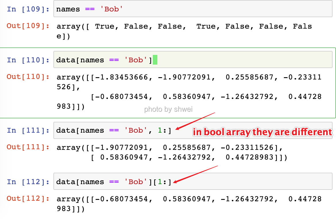
data[names == 'Bob']

array([[ 2.44492395, -1.52038895,  0.39391998, -0.31685538],
       [ 1.6580849 ,  0.45994775,  0.86858598, -0.7588714 ]])

# First dimension fetch data based on boolean
# Second dimension fectch data based on slice
data[names == 'Bob', 1:] 

array([[-1.52038895,  0.39391998, -0.31685538],
       [ 0.45994775,  0.86858598, -0.7588714 ]])

data[names == 'Bob'][1:]

array([[ 1.6580849 ,  0.45994775,  0.86858598, -0.7588714 ]])

data[names == 'Bob', 3]

array([-0.31685538, -0.7588714 ])

To select everything but ‘Bob’, you can either use != or negate the condition using ~

names != 'Bob'

array([False,  True,  True, False,  True,  True,  True])

data[~(names == 'Bob')]

array([[-0.08518141,  0.38465576, -0.59752249, -1.9550803 ],
       [-0.47663211, -0.23931735,  0.71509259,  0.11847852],
       [-0.17831281, -0.3973996 ,  0.48140504, -0.20286526],
       [ 0.02599393,  0.37176764, -0.83564336, -0.83812596],
       [-0.03231511, -1.66515562,  0.04271532,  0.55256624]])

Selecting two of the three names to combine mutiple boolean conditions, use boolean arithmetic operators like &(and) and |(or):

Note: The Python keywords and and or do not work with boolean arrays.

mask = (names == 'Bob') | (names == 'Will')

mask

array([ True, False,  True,  True,  True, False, False])

data1 = data[mask] # make a copy

data1

array([[ 2.44492395, -1.52038895,  0.39391998, -0.31685538],
       [-0.47663211, -0.23931735,  0.71509259,  0.11847852],
       [ 1.6580849 ,  0.45994775,  0.86858598, -0.7588714 ],
       [-0.17831281, -0.3973996 ,  0.48140504, -0.20286526]])

data1[1] = 0

data1

array([[ 2.44492395, -1.52038895,  0.39391998, -0.31685538],
       [ 0.        ,  0.        ,  0.        ,  0.        ],
       [ 1.6580849 ,  0.45994775,  0.86858598, -0.7588714 ],
       [-0.17831281, -0.3973996 ,  0.48140504, -0.20286526]])

data

array([[ 2.44492395, -1.52038895,  0.39391998, -0.31685538],
       [-0.08518141,  0.38465576, -0.59752249, -1.9550803 ],
       [-0.47663211, -0.23931735,  0.71509259,  0.11847852],
       [ 1.6580849 ,  0.45994775,  0.86858598, -0.7588714 ],
       [-0.17831281, -0.3973996 ,  0.48140504, -0.20286526],
       [ 0.02599393,  0.37176764, -0.83564336, -0.83812596],
       [-0.03231511, -1.66515562,  0.04271532,  0.55256624]])

Note: Selecting data from an array by boolean indexing always creates a copy of the data.
Set all of the negative values in data to 0

data < 0

array([[False,  True, False,  True],
       [ True, False,  True,  True],
       [ True,  True, False, False],
       [False, False, False,  True],
       [ True,  True, False,  True],
       [False, False,  True,  True],
       [ True,  True, False, False]])

data[data < 0] = 0

data

array([[2.44492395, 0.        , 0.39391998, 0.        ],
       [0.        , 0.38465576, 0.        , 0.        ],
       [0.        , 0.        , 0.71509259, 0.11847852],
       [1.6580849 , 0.45994775, 0.86858598, 0.        ],
       [0.        , 0.        , 0.48140504, 0.        ],
       [0.02599393, 0.37176764, 0.        , 0.        ],
       [0.        , 0.        , 0.04271532, 0.55256624]])

4.1.6 Fancy Indexing

Fancy indexing is a term adpoted by Numpy to describe indexing using integer arrays.

Case 1: Basic Indexing and Slicing

arr[2:]

array([  2,   3,   4,  12, 100,  12,   8,   9])

arr[0]

0

Case 2: Boolean Indexing

arr = np.array([1,3,4,5])
bool_ = np.array([True, False, True, False], dtype = np.bool)

bool_

array([ True, False,  True, False])

arr[bool_]

array([1, 4])

4.1.6.1 Key of Fancy Indexing

Case 3: Fancy Indexing

• Return a copy of original array
• To select out a subset of the rows in a particular order, you can simply pass a list or ndaray of integers specifying the desired order

arr = np.array([1,2,3,4])

arr[[2,3,1,0],] # [2,3,1,0] is a list

array([3, 4, 2, 1])

index_arr = np.array([3,2,0,1])

index_arr

array([3, 2, 0, 1])

arr[index_arr] # index_arr is a ndarray

array([4, 3, 1, 2])

I think Boolean Indexing is a special Fancy Indexing.

arr

array([1, 2, 3, 4])

arr[[1,2]] #(1,) (2,)

array([2, 3])

arr[[-1, -3],] #(-1,) (-3,)

array([4, 2])

arr = np.arange(32).reshape((8,4))

arr

array([[ 0,  1,  2,  3],
       [ 4,  5,  6,  7],
       [ 8,  9, 10, 11],
       [12, 13, 14, 15],
       [16, 17, 18, 19],
       [20, 21, 22, 23],
       [24, 25, 26, 27],
       [28, 29, 30, 31]])

# select each dimension
arr[[1,5,7,2],[0,3,1,2]] # (1,0) (5,3) (7,1) (2,2)

array([ 4, 23, 29, 10])

arr[[1,5,7,2]] # (1,:) (5,:) (7,:) (2,:)

array([[ 4,  5,  6,  7],
       [20, 21, 22, 23],
       [28, 29, 30, 31],
       [ 8,  9, 10, 11]])

# Can be understood as: first exchange the second dimension, and then select all the first dimensions
arr[[1,5,7,2]][:, [0,3,1,2]] 

array([[ 4,  7,  5,  6],
       [20, 23, 21, 22],
       [28, 31, 29, 30],
       [ 8, 11,  9, 10]])

4.1.7 Transposing Arrays and Swapping Axes

Transposing is a special form of reshaping which similarly returns a view on the underlying data without copying anything.

Transposing: arr[0, 1, 2] = arr.T[2,1,0] After transposing the axes is from dn to d1

arr = np.arange(24).reshape((2,3,4))

arr

array([[[ 0,  1,  2,  3],
        [ 4,  5,  6,  7],
        [ 8,  9, 10, 11]],

       [[12, 13, 14, 15],
        [16, 17, 18, 19],
        [20, 21, 22, 23]]])

arr[0,1,2]

6

arr size: $2*3*4$

arr.T size: $4*3*2$

arr_T = arr.T
arr.T # a view of arr

array([[[ 0, 12],
        [ 4, 16],
        [ 8, 20]],

       [[ 1, 13],
        [ 5, 17],
        [ 9, 21]],

       [[ 2, 14],
        [ 6, 18],
        [10, 22]],

       [[ 3, 15],
        [ 7, 19],
        [11, 23]]])

arr_T[0][1] = 3333

arr

array([[[   0,    1,    2,    3],
        [3333,    5,    6,    7],
        [   8,    9,   10,   11]],

       [[  12,   13,   14,   15],
        [3333,   17,   18,   19],
        [  20,   21,   22,   23]]])

arr_T[2][1][0] # arr_T is the array after arr transposing

6

Computing the inner matrix product $X^TX$ using np.dot

arr = np.random.randint(1, 4, size=(3,4))

arr

array([[3, 3, 2, 2],
       [1, 3, 2, 1],
       [2, 2, 3, 1]])

# inner matrix product
np.dot(arr.T, arr)

array([[14, 16, 14,  9],
       [16, 22, 18, 11],
       [14, 18, 17,  9],
       [ 9, 11,  9,  6]])

arr = np.arange(24).reshape((2,3,4))

arr # size 2*3*4

array([[[ 0,  1,  2,  3],
        [ 4,  5,  6,  7],
        [ 8,  9, 10, 11]],

       [[12, 13, 14, 15],
        [16, 17, 18, 19],
        [20, 21, 22, 23]]])

transpose change axes (0,1,2) to (1,0,2)

So for example the index (1,2,3) will be index(2,1,3)

arr.transpose(1,0,2) # size 2 * 3 * 4 

array([[[ 0,  1,  2,  3],
        [12, 13, 14, 15]],

       [[ 4,  5,  6,  7],
        [16, 17, 18, 19]],

       [[ 8,  9, 10, 11],
        [20, 21, 22, 23]]])

ndarray has the method swapaxes which takes a pair of axis numbers

arr # size 2*3*4

array([[[ 0,  1,  2,  3],
        [ 4,  5,  6,  7],
        [ 8,  9, 10, 11]],

       [[12, 13, 14, 15],
        [16, 17, 18, 19],
        [20, 21, 22, 23]]])

arr.swapaxes(1,2) # size 2*4*3  return a copy

array([[[ 0,  4,  8],
        [ 1,  5,  9],
        [ 2,  6, 10],
        [ 3,  7, 11]],

       [[12, 16, 20],
        [13, 17, 21],
        [14, 18, 22],
        [15, 19, 23]]])

arr[1,2,1]

21

arr.swapaxes(1,2)[1,1,2]

21

4.2 Universal Functions: Fast Element-wise Array Functions

A universal function, or ufunc, is a function that performs elementwise operations on data in ndarrays.You can think of them as fastvectorized wrappers for simple functions.

arr = np.arange(10)

arr

array([0, 1, 2, 3, 4, 5, 6, 7, 8, 9])

np.sqrt(arr)

array([0.        , 1.        , 1.41421356, 1.73205081, 2.        ,
       2.23606798, 2.44948974, 2.64575131, 2.82842712, 3.        ])

np.exp(arr)

array([1.00000000e+00, 2.71828183e+00, 7.38905610e+00, 2.00855369e+01,
       5.45981500e+01, 1.48413159e+02, 4.03428793e+02, 1.09663316e+03,
       2.98095799e+03, 8.10308393e+03])

x = np.random.randn(8)
y = np.random.randn(8)

x

array([ 0.60058561, -1.30032727, -1.17669429, -1.16293769,  1.6389972 ,
       -0.53815749, -0.14142643,  1.02354324])

y

array([-1.61302358, -0.354913  , -0.1137763 ,  0.08010182,  0.07466485,
       -1.39663575,  0.77496037,  1.75997402])

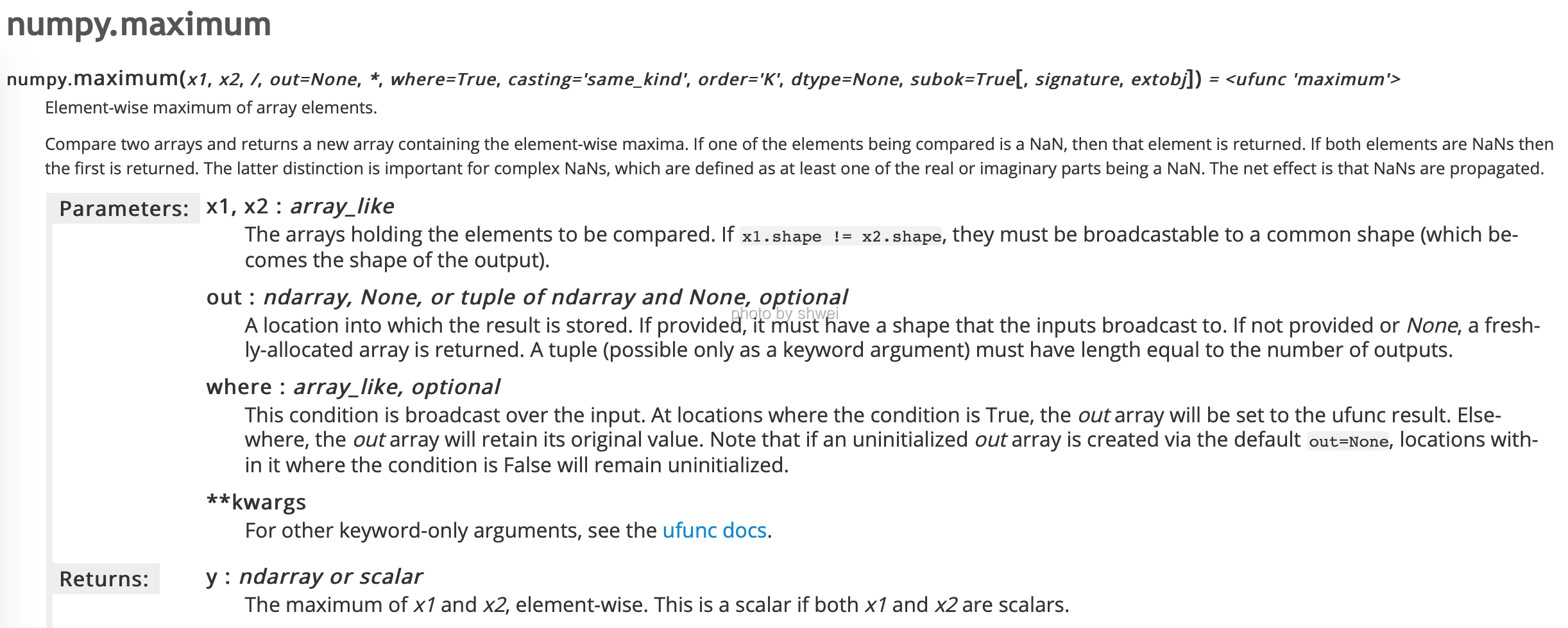
np.maximum(x, y)

array([ 0.60058561, -0.354913  , -0.1137763 ,  0.08010182,  1.6389972 ,
       -0.53815749,  0.77496037,  1.75997402])

arr = np.random.randn(7) * 5

arr

array([ 7.50554328, -0.61609252,  3.00616797, -6.02160661,  3.83440266,
       -6.53201864,  7.47775811])

remainder, whole_part = np.modf(arr)

remainder

array([ 0.50554328, -0.61609252,  0.00616797, -0.02160661,  0.83440266,
       -0.53201864,  0.47775811])

whole_part

array([ 7., -0.,  3., -6.,  3., -6.,  7.])

Universal Function accept a optional parameter out

arr 

array([ 7.50554328, -0.61609252,  3.00616797, -6.02160661,  3.83440266,
       -6.53201864,  7.47775811])

np.sqrt(arr, arr)

/usr/local/lib/python3.7/site-packages/ipykernel_launcher.py:1: RuntimeWarning: invalid value encountered in sqrt
  """Entry point for launching an IPython kernel.





array([2.73962466,        nan, 1.73383043,        nan, 1.95816308,
              nan, 2.73454898])

arr

array([2.73962466,        nan, 1.73383043,        nan, 1.95816308,
              nan, 2.73454898])

arr = np.random.randn(10)

arr

array([-0.40366505, -1.98954395, -1.05020216, -0.01818649, -1.08323461,
        0.0976977 , -1.45609853, -0.99915274, -1.88666922, -0.10298285])

np.sign(arr)

array([-1., -1., -1., -1., -1.,  1., -1., -1., -1., -1.])

arr1 = np.array(range(10))
arr2 = np.arange(1,11)

arr1

array([0, 1, 2, 3, 4, 5, 6, 7, 8, 9])

arr2

array([ 1,  2,  3,  4,  5,  6,  7,  8,  9, 10])

np.subtract(arr1, arr2)

array([-1, -1, -1, -1, -1, -1, -1, -1, -1, -1])

np.copysign(arr, arr2) # copy arr2's sign to arr

array([0.40366505, 1.98954395, 1.05020216, 0.01818649, 1.08323461,
       0.0976977 , 1.45609853, 0.99915274, 1.88666922, 0.10298285])

4.2.1 API https://www.geeksforgeeks.org/ , Google, Dash

You don’t need to remember all the function. When you need it, just search the function in Google or Dash.

4.2.2 A listing of available ufuncs

Table 4-3. Unary ufuncs

Function	Description
abs, fabs	Compute the absolute value element-wise for integer, floating point, or complex values.Use fabs as a faster alternative for non-complex-valued data
sqrt	Compute the square root of each element. Equivalent to arr ** 0.5
square	Compute the square of each element. Equivalent to arr ** 2
exp	Compute the exponent $e^x$ of each element
log, log10, log2, log1p	Natural logarithm (base e), log base 10, log base 2, and log(1 + x), respectively
sign	Compute the sign of each element: 1 (positive), 0 (zero), or -1 (negative)
ceil	Compute the ceiling of each element, i.e. the smallest integer greater than or equal to each element
floor	Compute the floor of each element, i.e. the largest integer less than or equal to each element
rint	Round elements to the nearest integer, preserving the dtype
modf	Return fractional and integral parts of array as separate array
isnan	Return boolean array indicating whether each value is NaN (Not a Number)
isfinite, isinf	Return boolean array indicating whether each element is finite (non-inf, non-NaN) or infinite, respectively
cos, cosh, sin, sinh, tan, tanh	Regular and hyperbolic trigonometric functions
arccos, arccosh, arcsin, arcsinh, arctan, arctanh	Inverse trigonometric functions
logical_not	Compute truth value of not x element-wise. Equivalent to -arr

Table 4-4. Binary universal functions

Function	Description
add	Add corresponding elements in arrays
subtract	Subtract elements in second array from first array
multiply	Multiply array elements
divide, floor_divide	Divide or floor divide (truncating the remainder)
power	Raise elements in first array to powers indicated in second array
maximum, fmax	Element-wise maximum. fmax ignores NaN
minimum, fmin	Element-wise minimum. fmin ignores NaN
mod	Element-wise modulus (remainder of division)
copysign	Copy sign of values in second argument to values in first argument
greater, greater_equal, less, less_equal, equal, not_equal	Perform element-wise comparison, yielding boolean array. Equivalent to infix operators >, >=, <, <=, ==, !=
logical_and,logical_or, logical_xor	Compute element-wise truth value of logical operation. Equivalent to infix operators &, |, ^

4.3 Data Processing Using Arrays

4.3.0 np.meshgrid()

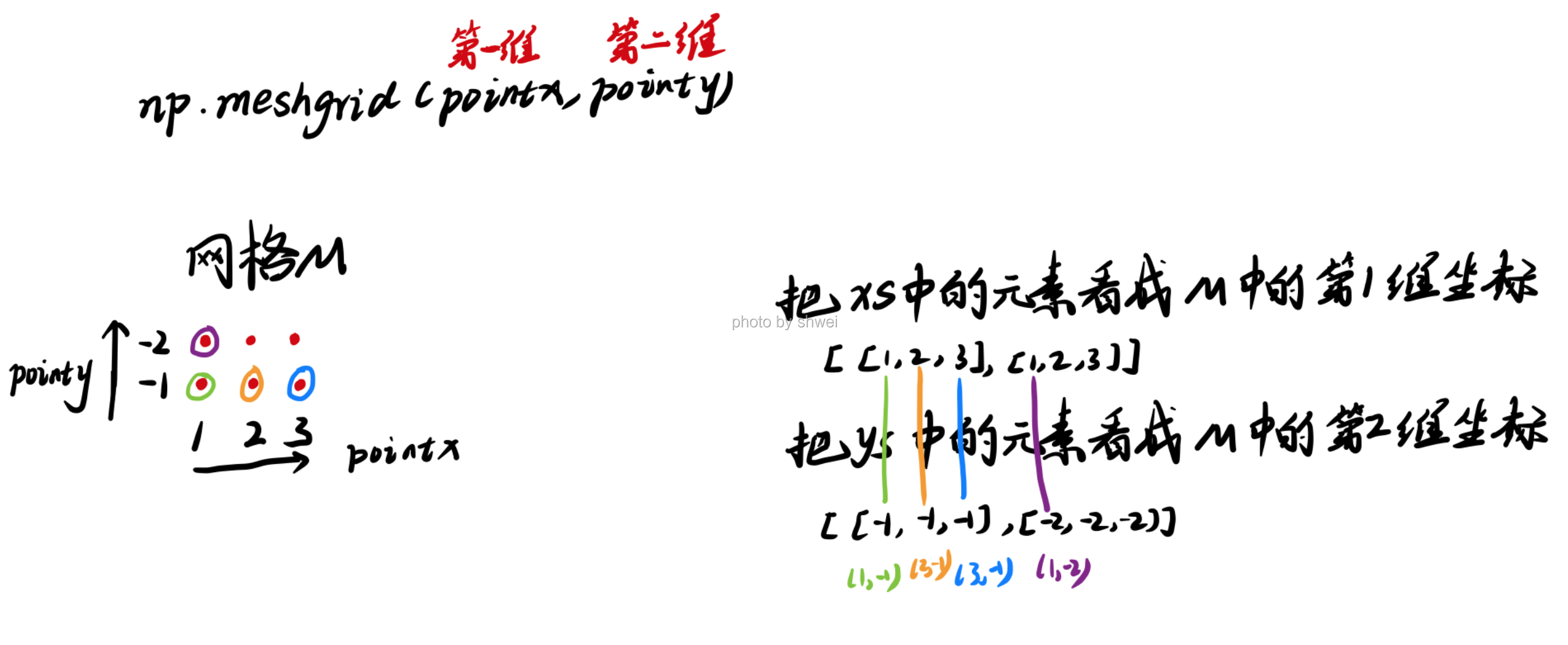
The np.meshgrid function takes two 1D arrays and produces two 2D matrices corresponding to all pairs of (x, y) in the two arrays:

pointx = np.array([1,2,3])
pointy = np.array([-1,-2])
matrices = np.meshgrid(pointx,pointy)

matrices

[array([[1, 2, 3],
        [1, 2, 3]]),
 array([[-1, -1, -1],
        [-2, -2, -2]])]

xs, ys = np.meshgrid(pointx,pointy)

xs

array([[1, 2, 3],
       [1, 2, 3]])

ys

array([[-1, -1, -1],
       [-2, -2, -2]])

How to understand np.meshgrid()

z = np.sqrt(xs ** 2 + ys ** 2)

z

array([[1.41421356, 2.23606798, 3.16227766],
       [2.23606798, 2.82842712, 3.60555128]])

import matplotlib.pyplot as plt

plt.imshow(z, cmap = plt.cm.gray); plt.colorbar()
plt.title("Image plot of $\sqrt{x ^ 2 + y ^ 2}$ for a grid of values")

Text(0.5, 1.0, 'Image plot of $\\sqrt{x ^ 2 + y ^ 2}$ for a grid of values')

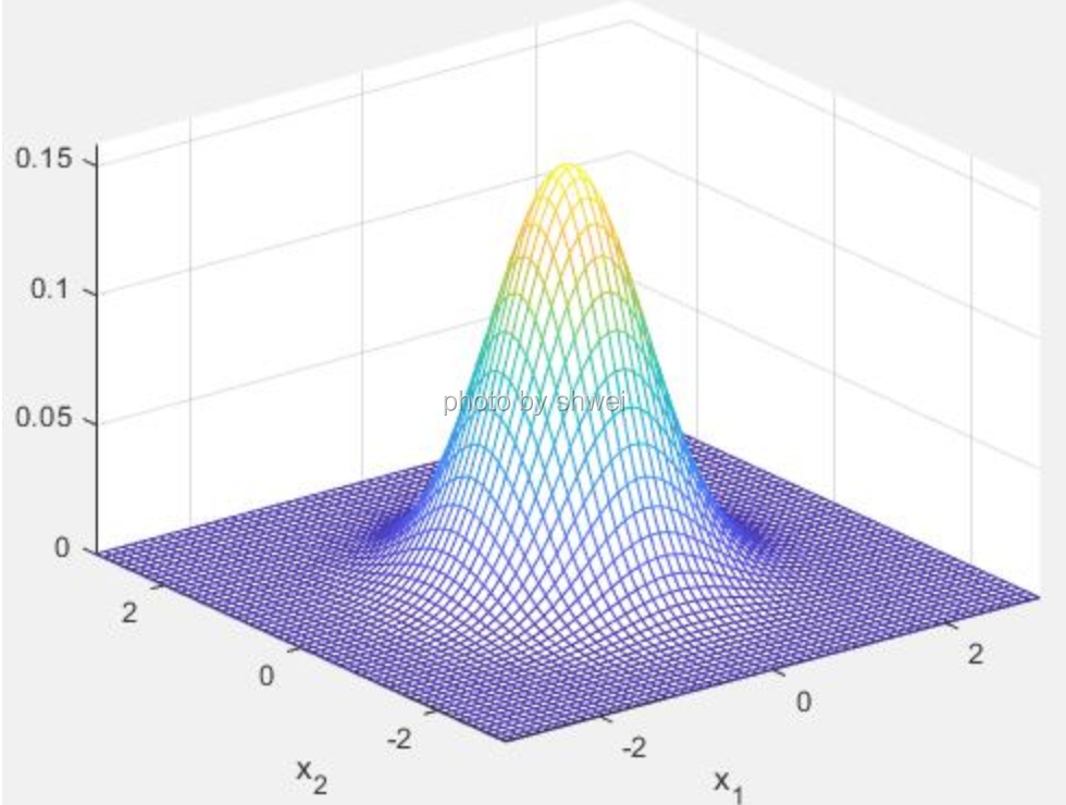
[外链图片转存失败,源站可能有防盗链机制,建议将图片保存下来直接上传(img-cQ7da8pB-1583481497049)(output_203_1.png)]

Figure 4-3. Plot of function evaluated on grid

Here I used the matplotlib function imshow to create an image plot
from a 2D array of function values.

4.3.1 Expressing Conditional Logic as Array Operations

The numpy.where function is a vectorized version of the ternary expression x if condtion else y

xarr = np.array([1,2,3,4])
yarr = np.array([-1,-2,-3,-4])
cond = np.array([True, False, True, True])

result = [x if c else y for x, y, c in zip(xarr, yarr, cond)]

result

[1, -2, 3, 4]

This has multiple problems. First, it will not be very fast for large arrays (because all the work is being done in pure Python). Secondly, it will not work with multidimensional arrays.

With np.where you can write this very concisely

result = np.where(cond, xarr, yarr)

result

array([ 1, -2,  3,  4])

The second and third arguments to np.where don’t need to be arrays.A typical use of where in data analysis is to produce a new array of values based on another array.

arr = np.random.randn(4,3)

arr

array([[-0.01139784,  0.40169215, -0.38962953],
       [ 0.55216629,  0.48477693, -0.06194546],
       [ 0.54855517,  0.17247726, -0.74025193],
       [-0.39221758,  0.24833925,  1.15466766]])

np.where(arr > 0, arr, -2)

array([[-2.        ,  0.40169215, -2.        ],
       [ 0.55216629,  0.48477693, -2.        ],
       [ 0.54855517,  0.17247726, -2.        ],
       [-2.        ,  0.24833925,  1.15466766]])

The arrays passed to where can be more than just equal sizes array or scales.

4.3.2 Mathematical and Statistical Methods

arr = np.random.randn(5,4) # normally-distributed data

arr 

array([[-1.7669711 ,  0.23033242, -0.66245059, -1.10571503],
       [ 0.17697343,  0.09412475,  2.31777073, -0.44555725],
       [-0.62426573,  1.75648072,  0.95977683, -0.61619976],
       [-0.49642721,  0.45912091,  1.26163226,  0.06395789],
       [ 1.66048345,  0.34056885, -1.54478641, -1.04533225]])

arr = np.arange(15).reshape(5, 3)

arr

array([[ 0,  1,  2],
       [ 3,  4,  5],
       [ 6,  7,  8],
       [ 9, 10, 11],
       [12, 13, 14]])

arr.mean() # Average of all numbers

7.0

arr.sum() # Sum of all numbers

105

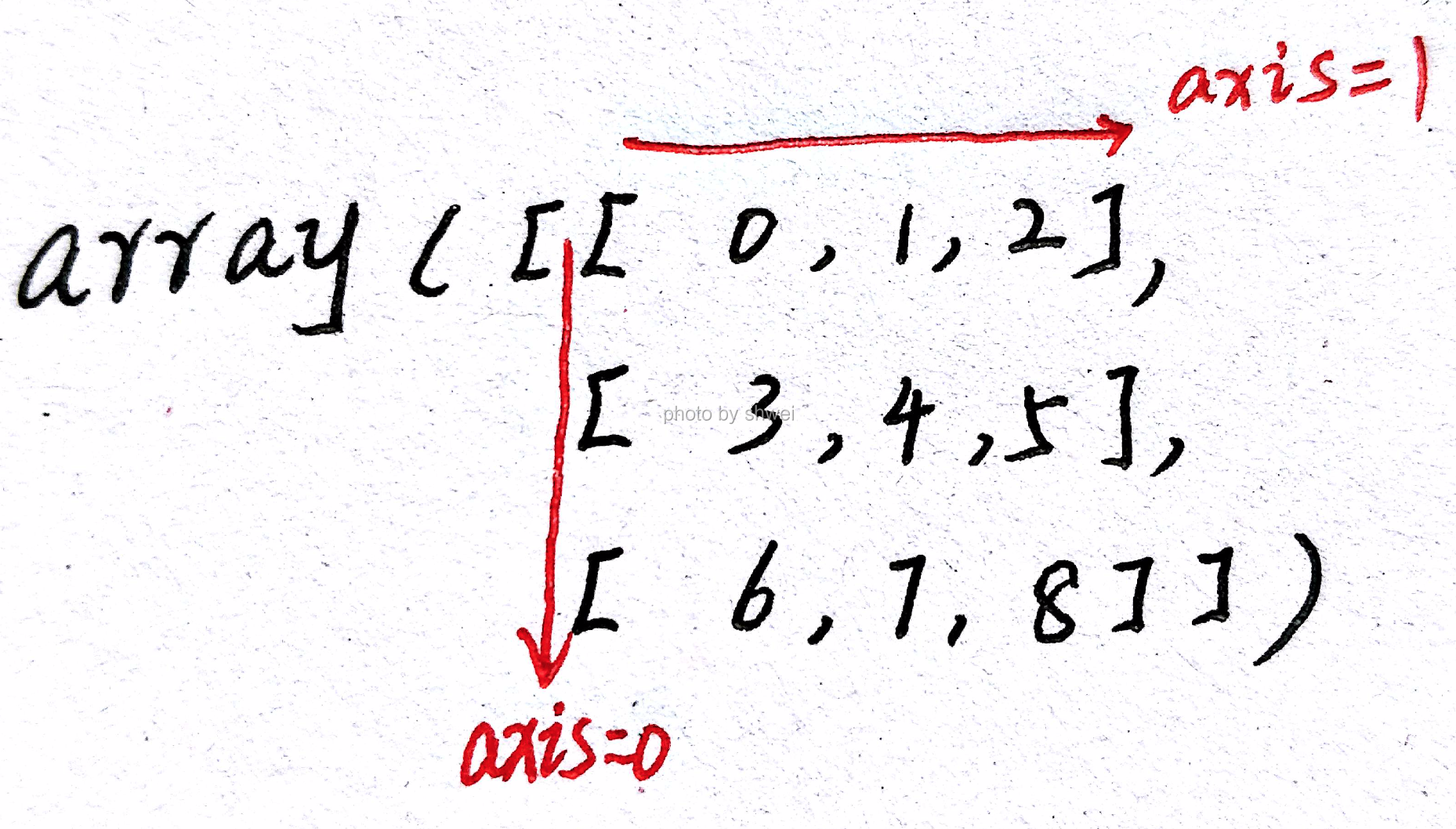
Functions like mean and sum take an optional axis argument
which computes the statistic over the given axis, resulting in an array
with one fewer dimension, or compressing the given axis

arr

array([[ 0,  1,  2],
       [ 3,  4,  5],
       [ 6,  7,  8],
       [ 9, 10, 11],
       [12, 13, 14]])

# arr[3][1] == 10
# axis 1 is the direction 0->1->2 here
arr.mean(axis = 1) # compress axis 1 and here is (5, 3)‘s 3

array([ 1.,  4.,  7., 10., 13.])

arr.sum(axis = 0)

array([30, 35, 40])

arr.sum(0)

array([30, 35, 40])

arr.min(1) # dimension reduced

array([ 0,  3,  6,  9, 12])

arr.argmax(1) # Indices of maximum elements, respective

array([2, 2, 2, 2, 2])

arr = np.arange(10)

arr

array([0, 1, 2, 3, 4, 5, 6, 7, 8, 9])

arr.cumsum()

array([ 0,  1,  3,  6, 10, 15, 21, 28, 36, 45])

arr = np.arange(9).reshape(3,3)

arr

array([[0, 1, 2],
       [3, 4, 5],
       [6, 7, 8]])

arr.cumsum(0)

array([[ 0,  1,  2],
       [ 3,  5,  7],
       [ 9, 12, 15]])

arr.cumprod(axis = 1)

array([[  0,   0,   0],
       [  3,  12,  60],
       [  6,  42, 336]])

Table 4-5. Basic array statistical methods

Method	Description
sum	Sum of all the elements in the array or along an axis. Zero-length arrays have sum 0.
mean	Arithmetic mean. Zero-length arrays have NaN mean.
std, var	Standard deviation and variance, respectively, with optional degrees of freedom adjustment (default denominator n).
min, max	Minimum and maximum.
argmin, argmax	Indices of minimum and maximum elements, respectively.
cumsum	Cumulative sum of elements starting from 0
cumprod	Cumulative product of elements starting from 1

4.3.3 Methods for Boolean Arrays

Boolean values are coerced to 1(True) and 0(False) in the above methods.

arr = np.random.randn(100)

(arr > 0).sum() # Number of positive values

46

There are two additional methods, any and all, useful especially for boolean
arrays.

any tests whether one or more values in an array is True, while all checks if every value
is True

bools = np.array([True, False, False, False])

bools.any()

True

bools.all()

False

bools.sum()

1

4.3.4 Sorting

Like Python’s built-in list type, NumPy arrays can be sorted in-place using the sort method

arr = np.random.randn(8)

arr

array([-0.05645386, -0.36224588, -1.29498701, -0.30476409, -0.46770012,
        1.20385542,  1.47953717, -0.20565266])

arr.sort()

arr

array([-1.29498701, -0.46770012, -0.36224588, -0.30476409, -0.20565266,
       -0.05645386,  1.20385542,  1.47953717])

4.3.5 Unique and Other Set Logic

NumPy has some basic set operations for one-dimensional ndarrays. Probably
the most commonly used one is np.unique, which returns the sorted unique values in an array

names = np.array(['Bob', 'Will','Joe',  'Bob', 'Will'])

np.unique(names)

array(['Bob', 'Joe', 'Will'], dtype='<U4')

names

array(['Bob', 'Will', 'Joe', 'Bob', 'Will'], dtype='<U4')

ints = np.array([3,3,3,2,2,1,2,3,5])

np.unique(ints)

array([1, 2, 3, 5])

Constract np.unique with the pure Python alternative

sorted(set(names))

['Bob', 'Joe', 'Will']

Another function, np.in1d, tests membership of the values in one array in another, returning a boolean array.

values = np.array([3,2,31,44,34,5])

np.in1d(values, [2,3])

array([ True,  True, False, False, False, False])

Table 4-6. Array set operations

Method	Description
unique(x)	Compute the sorted, unique elements in x
intersect1d(x, y)	Compute the sorted, common elements in x and y
union1d(x, y)	Compute the sorted union of elements
in1d(x, y)	Compute a boolean array indicating whether each element of x is contained in y
setdiff1d(x, y)	Set difference, elements in x that are not in y
setxor1d(x, y)	Set symmetric differences; elements that are in either of the arrays, but not both

4.4 File Input and Output with Arrays

NumPy is able to save and load data to and from disk either in text or binary format.
In later chapters you will learn about tools in pandas for reading tabular data into
memory.

4.5 Linear Algebra

Linear algebra, like matrix multiplication, decompostions, determinants, and other square matrix math, is
an important part of any array library.

Unlike some languages like MATLAB, multiplying two-dimensional arrays with * is an element-wise product instead of a matrix dot product.

As such, there is a function dot, both an array
method, and a function in the numpy namespace

x = np.array([[1,2,3],[4,5,6]])

x

array([[1, 2, 3],
       [4, 5, 6]])

x * x

array([[ 1,  4,  9],
       [16, 25, 36]])

y = np.arange(6).reshape(3,2)

y

array([[0, 1],
       [2, 3],
       [4, 5]])

x.dot(y) # ndarray function

array([[16, 22],
       [34, 49]])

np.dot(x,y) # a function in numpy namespace

array([[16, 22],
       [34, 49]])

x

array([[1, 2, 3],
       [4, 5, 6]])

x @ np.ones(3) # @ is also used in a matrix dot product

array([ 6., 15.])

numpy.linalg(linear algebra) has a standard set of matrix decompositions and things like inverse and determinant. These are implemented under the hood using the same industry-standard Fortran libraries used in other languages like MATLAB and R, such as like BLAS,LAPACK, or possibly(depending on your NumPy build) the Intel MKL

更新标准写法是：from numpy.linalg import inv, qr，这样求逆就直接写inv(matrix)

import numpy.linalg as npla # npla是我自己取的名，不规范
matrix = np.random.randn(4,4)

npla.inv(matrix)

array([[-46.76938498, -86.35815947, 129.96228838, -32.95425663],
       [-22.31060821, -41.56709931,  62.01812792, -15.25370697],
       [-20.35569284, -37.11177381,  54.70106286, -14.5358842 ],
       [-30.82139292, -54.49869152,  81.79616404, -21.54068957]])

arr = matrix.dot(npla.inv(matrix)) # np.dot(matrix, npla.inv(matrix))

arr

array([[ 1.00000000e+00, -5.73321716e-15, -4.64130813e-15,
        -1.34965101e-16],
       [ 1.03102760e-15,  1.00000000e+00, -1.13084465e-14,
         6.16824551e-16],
       [-6.92801263e-15, -9.06342203e-15,  1.00000000e+00,
        -3.46276746e-15],
       [ 1.61273987e-17, -4.13259316e-15, -9.54630608e-15,
         1.00000000e+00]])

np.round(arr, 2) # decimals=2

array([[ 1., -0., -0., -0.],
       [ 0.,  1., -0.,  0.],
       [-0., -0.,  1., -0.],
       [ 0., -0., -0.,  1.]])

Table 4-7. Commonly-used numpy.linalg functions

Function	Description
diag	Return the diagonal (or off-diagonal) elements of a square matrix as a 1D array, or convert a 1D array into a square matrix with zeros on the off-diagonal
dot	Matrix multiplication
trace	Compute the sum of the diagonal elements
det	Compute the matrix determinant
eig	Compute the eigenvalues and eigenvectors of a square matrix
inv	Compute the inverse of a square matrix
pinv	Compute the Moore-Penrose pseudo-inverse inverse of a square matrix
qr	Compute the QR decomposition
svd	Compute the singular value decomposition (SVD)
solve	Solve the linear system Ax = b for x, where A is a square matrix
lstsq	Compute the least-squares solution to y = Xb

4.6 Random Number Generation

The numpy.random module supplements the built-in Python random with functions for efficiently generating whole arrays of sample values from many kinds of probabiliry distributions.

Table 4-8. Partial list of numpy.random functions

Function	Description
seed	Seed the random number generator
permutation	Return a random permutation of a sequence, or return a permuted range
shuffle	Randomly permute a sequence in place
rand	Draw samples from a uniform distribution
randint	Draw random integers from a given low-to-high range
randn	Draw samples from a normal distribution with mean 0 and standard deviation 1 (MATLAB-like interface)
binomial	Draw samples a binomial distribution
normal	Draw samples from a normal (Gaussian) distribution
beta	Draw samples from a beta distribution
chisquare	Draw samples from a chi-square distribution
gamma	Draw samples from a gamma distribution
uniform	Draw samples from a uniform [0, 1) distribution

samples = np.random.normal(size = (4,4))

np.round(samples,4)

array([[-0.4422, -0.1181, -1.1577,  0.4524],
       [ 0.923 ,  1.8407,  0.1605, -0.9159],
       [ 0.7133, -0.0398, -1.3522, -1.1874],
       [-0.4133,  0.7873, -0.9728, -0.9143]])

Python’s built-in random module by constrast only samples one value at a time. As you can see from this benchmark, numpy.random is well over an order of magnitude faster for generating very large samples

from random import normalvariate
N = 1000000

%timeit sample = [normalvariate(0,1) for _ in range(N)]

1.16 s ± 99.4 ms per loop (mean ± std. dev. of 7 runs, 1 loop each)

%timeit np.random.normal(size = N)

33 ms ± 1.39 ms per loop (mean ± std. dev. of 7 runs, 10 loops each)

They’re actually what’s known as " pseudo random numbers, " generated by algorithms.

4.6.1 random.random((m,n))

The function parameter is a tuple

Generate random numbers from 0 to 1

import numpy as np
data = np.random.random((2,5))

# Show the variable
data

array([[0.87481527, 0.11475954, 0.52484471, 0.86935258, 0.09528812],
       [0.15106181, 0.12227048, 0.81898961, 0.33022438, 0.94330205]])

# Print the variable  
print(data)

[[0.87481527 0.11475954 0.52484471 0.86935258 0.09528812]
 [0.15106181 0.12227048 0.81898961 0.33022438 0.94330205]]

data * 10

array([[8.74815275, 1.14759543, 5.24844707, 8.69352576, 0.9528812 ],
       [1.51061807, 1.22270479, 8.18989614, 3.30224382, 9.43302047]])

print(data + data)

[[1.74963055 0.22951909 1.04968941 1.73870515 0.19057624]
 [0.30212361 0.24454096 1.63797923 0.66044876 1.88660409]]

ndim: the first dimension

data.ndim

2

shape: a tuple indicating the size of each dimension

data.shape

(2, 5)

data_ = np.array([1,2,3])
data_.shape # (3,) Only have one dimension

(3,)

dtype: decribe the data type of the array

data.dtype

dtype('float64')

data2 = np.random.random(9)
data2

array([0.0155825 , 0.80244718, 0.14901417, 0.42191698, 0.60644615,
       0.37694115, 0.2821992 , 0.97835977, 0.08436808])

4.6.2 random.randint(1,8, size = (3,2))

Generate random integer from 1 to 8, left close and right open

data_randint = np.random.randint(1,8,size = (3, 2))
data_randint

array([[7, 6],
       [7, 7],
       [1, 2]])

4.6.3 random.randn(d1, d2, d3, …)

randn generates a matrix filled with random floats sampled from a univarite “normal” distribution of mean 0 and variance 1

Notes:
For random samples from $N(\sigma, \mu ^ 2)$,use:

sigma * np.random.randn(d1, ) + mu

# N(1, 6.25)
data_normal_distribution = 1 * np.random.randn(2,3) + 2.5
data_normal_distribution

array([[4.03463856, 5.86698859, 2.59342223],
       [2.18876421, 1.66281754, 1.51047393]])

NumPy Summay

The biggest benefit of NumPy arrays is the use of simple array expressions to complete a variety of data manipulation tasks without the need to write some loops.

• Basic Indexing, Slicing, arr.T return view
• Boolean Indexing, Fancy Indexing, arr.swapaxes return copy

arr2d

array([[1, 0, 0],
       [4, 0, 0],
       [7, 8, 9]])

arr_test = arr2d[:2, 1:] # return view
arr_test = 0 # This will change the original arr2d

arr2d

array([[1, 0, 0],
       [4, 0, 0],
       [7, 8, 9]])

• , locate the dimension
• : keep in same dimension (Slicing)
• [2,3,1] choose some in this dimension (Fancy Indexing)

arr2d[1,0]

4

arr2d[1,]

array([4, 0, 0])

arr2d[:2,0]

array([1, 4])

arr2d[:2,:1] 

array([[1],
       [4]])

arr2d[[2,1]]

array([[7, 8, 9],
       [4, 0, 0]])

How to locate number 5

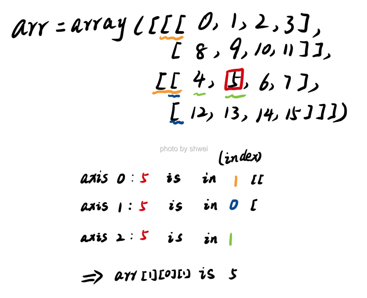
Change axis

Example 1:
arr size: 2∗3∗4
arr.T size: 4∗3∗2

old:(0,1,2) = 6
now:(2,1,0) = 6