Autor: Tarun Gupta
deephub tradução Grupo: Meng Xiangjie
Neste artigo, vamos olhar para usar NumPy como um programa escrito em Python3 biblioteca de processamento de dados para aprender a implementar (lote) de regressão linear usando o método do gradiente de descida.
Vou explicar gradualmente o princípio de funcionamento e com o princípio de cada parte do código do código.
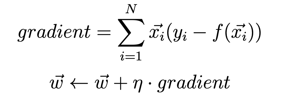
Vamos utilizar esta fórmula para calcular o gradiente.
Aqui, x (i) é um vector de um ponto, em que N é o tamanho do conjunto de dados. n (eta) é a nossa taxa de aprendizagem. y (i) é um vector de saída de destino. f (x) é definido como o vector f (x) = Soma (w * x) de uma função de regressão linear, onde sigma é a função de soma. Além disso, vamos considerar a diferença inicial w0 = 0 e tal que x0 = 1. Todos os pesos são inicializados a 0.
Neste método, foi utilizada a soma da função perda erro quadrado.
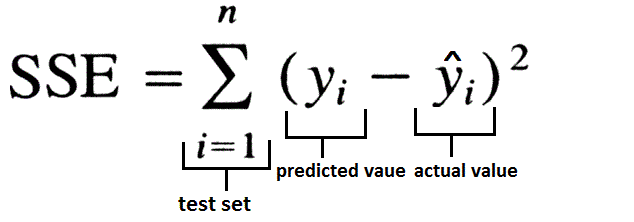
Só que SSE é inicializado para zero, vamos gravar as mudanças em cada iteração do SSE, e comparados com um valor limite previsto antes da execução do programa. Se SSE está abaixo do limite, o programa sai.
Neste programa, nós fornecemos três entradas a partir da linha de comando. São eles:
-
limite - o valor limite, antes dos termina algoritmo, a perda deve ser abaixo deste limiar.
-
dados - conjuntos de dados de posição.
-
learningRate - taxa de aprendizagem método de gradiente de descida.
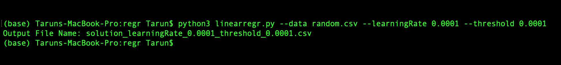
Portanto, o início do programa deve ficar assim:
python3 linearregr.py — data random.csv — learningRate 0.0001 — threshold 0.0001
Antes de mergulhar no código identificamos última coisa, a saída do programa seria a seguinte:
iteration_number,weight0,weight1,weight2,...,weightN,sum_of_squared_errors
O programa inclui seis partes, uma por uma, vemos.
módulo de importação
import argparse # to read inputs from command line
import csv # to read the input data set file
import numpy as np # to work with the data set
inicialização parte
# initialise argument parser and read arguments from command line with the respective flags and then call the main() functionif __name__ == '__main__':
    parser = argparse.ArgumentParser()
    parser.add_argument("-d", "--data", help="Data File")
    parser.add_argument("-l", "--learningRate", help="Learning Rate")
    parser.add_argument("-t", "--threshold", help="Threshold")
    main()
parte principal função
def main():
    args = parser.parse_args()
    file, learningRate, threshold = args.data, float(
        args.learningRate), float(args.threshold) # save respective command line inputs into variables

    # read csv file and the last column is the target output and is separated from the input (X) as Y
    with open(file) as csvFile:
        reader = csv.reader(csvFile, delimiter=',')
        X = []
        Y = []
        for row in reader:
            X.append([1.0] + row[:-1])
            Y.append([row[-1]])

    # Convert data points into float and initialise weight vector with 0s.
    n = len(X)
    X = np.array(X).astype(float)
    Y = np.array(Y).astype(float)
    W = np.zeros(X.shape[1]).astype(float)
    # this matrix is transposed to match the necessary matrix dimensions for calculating dot product
    W = W.reshape(X.shape[1], 1).round(4)

    # Calculate the predicted output value
    f_x = calculatePredicatedValue(X, W)

    # Calculate the initial SSE
    sse_old = calculateSSE(Y, f_x)

    outputFile = 'solution_' + \
                 'learningRate_' + str(learningRate) + '_threshold_' \
                 + str(threshold) + '.csv'
    '''
        Output file is opened in writing mode and the data is written in the format mentioned in the post. After the
        first values are written, the gradient and updated weights are calculated using the calculateGradient function.
        An iteration variable is maintained to keep track on the number of times the batch linear regression is executed
        before it falls below the threshold value. In the infinite while loop, the predicted output value is calculated
        again and new SSE value is calculated. If the absolute difference between the older(SSE from previous iteration)
        and newer(SSE from current iteration) SSE is greater than the threshold value, then above process is repeated.
        The iteration is incremented by 1 and the current SSE is stored into previous SSE. If the absolute difference
        between the older(SSE from previous iteration) and newer(SSE from current iteration) SSE falls below the
        threshold value, the loop breaks and the last output values are written to the file.
    '''
    with open(outputFile, 'w', newline='') as csvFile:
        writer = csv.writer(csvFile, delimiter=',', quoting=csv.QUOTE_NONE, escapechar='')
        writer.writerow([*[0], *["{0:.4f}".format(val) for val in W.T[0]], *["{0:.4f}".format(sse_old)]])

        gradient, W = calculateGradient(W, X, Y, f_x, learningRate)

        iteration = 1
        while True:
            f_x = calculatePredicatedValue(X, W)
            sse_new = calculateSSE(Y, f_x)

            if abs(sse_new - sse_old) > threshold:
                writer.writerow([*[iteration], *["{0:.4f}".format(val) for val in W.T[0]], *["{0:.4f}".format(sse_new)]])
                gradient, W = calculateGradient(W, X, Y, f_x, learningRate)
                iteration += 1
                sse_old = sse_new
            else:
                break
        writer.writerow([*[iteration], *["{0:.4f}".format(val) for val in W.T[0]], *["{0:.4f}".format(sse_new)]])
    print("Output File Name: " + outputFile
função principal do processo é como se segue:
- A linha de comando correspondente na entrada para uma variável
- Lendo o arquivo CSV, o último é uma saída de destino, e a entrada (armazenados como X) e armazenado como Y separado
- Converter o ponto de dados de ponto flutuante de inicialização vector de pesos para os 0s
- Use calculatePredicatedValue funcionar para calcular o valor previsto da saída
- função SSE usadas para calcular o calculateSSE inicial
- O arquivo de saída é aberto no modo de gravação, os dados são gravados no formato mencionado no artigo. Depois de escrever o primeiro valor, e usando a função gradiente de cálculo calculateGradient peso atualizado. número variável de repetições realizado para determinar a regressão linear realizado em modo descontínuo antes valores da função perda abaixo de um limiar. Enquanto num ciclo infinito, mais uma vez calculado o valor de saída previsto, e o cálculo de um novo valor de SSE. Se o velho (iteração anterior de SSE) ea mais recente a diferença absoluta entre (SSE da iteração atual) é maior que o valor limite, em seguida, repita o processo. Aumentar o número de iterações 1, SSE está armazenado em SSE anterior. Se o mais velho (iteração anterior de SSE) ea mais recente a diferença absoluta entre o (iteração atual do SSE) está abaixo do limite, o ciclo é interrompido, e o valor da produção final escrito para o arquivo.
calculatePredicatedValuefunção
Aqui, o produto é calculada através da realização da matriz de saída e de entrada previsto X W representa os pontos de matriz de peso.
# dot product of X(input) and W(weights) as numpy matrices and returning the result which is the predicted output
def calculatePredicatedValue(X, W):
    f_x = np.dot(X, W)
    return f_x
calculateGradientfunção
Gradiente calculada utilizando uma fórmula primeiro mencionada no artigo e actualizar os pesos.
def calculateGradient(W, X, Y, f_x, learningRate):
    gradient = (Y - f_x) * X
    gradient = np.sum(gradient, axis=0)
    temp = np.array(learningRate * gradient).reshape(W.shape)
    W = W + temp
    return gradient, W
calculateSSEfunção
SSE é calculado utilizando a equação acima.
def calculateSSE(Y, f_x):
    sse = np.sum(np.square(f_x - Y))
    return sse
Agora, leia o código completo. Vamos olhar os resultados da implementação do programa.
Isto é como a saída:
| 0 |
0.0000 |
0.0000 |
0.0000 |
7475.3149 |
| |
|
|
|
|
| 1 |
-0,0940 |
-0,5376 |
-0,2592 |
2111.5105 |
| |
|
|
|
|
| 2 |
-0,1789 |
-0,7849 |
-0,3766 |
880.6980 |
| |
|
|
|
|
| 3 |
-0,2555 |
-0,8988 |
-0,4296 |
538.8638 |
| |
|
|
|
|
| 4 |
-0,3245 |
-0,9514 |
-0,4533 |
399.8092 |
| |
|
|
|
|
| 5 |
-0,3867 |
-0,9758 |
-0,4637 |
316.1682 |
| |
|
|
|
|
| 6 |
-0,4426 |
-0,9872 |
-0,4682 |
254.5126 |
| |
|
|
|
|
| 7 |
-0,4930 |
-0,9926 |
-0,4699 |
205.8479 |
| |
|
|
|
|
| 8 |
-0,5383 |
-0,9952 |
-0,4704 |
166.6932 |
| |
|
|
|
|
| 9 |
-0,5791 |
-0,9966 |
-0,4704 |
135.0293 |
| |
|
|
|
|
| 10 |
-0,6158 |
-0,9973 |
-0,4702 |
109.3892 |
| |
|
|
|
|
| 11 |
-0,6489 |
-0,9978 |
-0,4700 |
88,6197 |
| |
|
|
|
|
| 12 |
-0,6786 |
-0,9981 |
-0,4697 |
71,7941 |
| |
|
|
|
|
| 13 |
-0,7054 |
-0,9983 |
-0,4694 |
58,1631 |
| |
|
|
|
|
| 14 |
-0,7295 |
-0,9985 |
-0,4691 |
47,1201 |
| |
|
|
|
|
| 15 |
-0,7512 |
-0,9987 |
-0,4689 |
38,1738 |
| |
|
|
|
|
| 16 |
-0,7708 |
-0,9988 |
-0.4687 |
30.9261 |
| |
|
|
|
|
| 17 |
-0.7883 |
-0.9989 |
-0.4685 |
25.0544 |
| |
|
|
|
|
| 18 |
-0.8042 |
-0.9990 |
-0.4683 |
20.2975 |
| |
|
|
|
|
| 19 |
-0.8184 |
-0.9991 |
-0.4681 |
16.4438 |
| |
|
|
|
|
| 20 |
-0.8312 |
-0.9992 |
-0.4680 |
13.3218 |
| |
|
|
|
|
| 21 |
-0.8427 |
-0.9993 |
-0.4678 |
10.7925 |
| |
|
|
|
|
| 22 |
-0.8531 |
-0.9994 |
-0.4677 |
8.7434 |
| |
|
|
|
|
| 23 |
-0.8625 |
-0.9994 |
-0.4676 |
7.0833 |
| |
|
|
|
|
| 24 |
-0.8709 |
-0.9995 |
-0.4675 |
5.7385 |
| |
|
|
|
|
| 25 |
-0.8785 |
-0.9995 |
-0.4674 |
4.6490 |
| |
|
|
|
|
| 26 |
-0.8853 |
-0.9996 |
-0.4674 |
3.7663 |
| |
|
|
|
|
| 27 |
-0.8914 |
-0.9996 |
-0.4673 |
3.0512 |
| |
|
|
|
|
| 28 |
-0.8969 |
-0.9997 |
-0.4672 |
2.4719 |
| |
|
|
|
|
| 29 |
-0.9019 |
-0.9997 |
-0.4672 |
2.0026 |
| |
|
|
|
|
| 30 |
-0.9064 |
-0.9997 |
-0.4671 |
1.6224 |
| |
|
|
|
|
| 31 |
-0.9104 |
-0.9998 |
-0.4671 |
1.3144 |
| |
|
|
|
|
| 32 |
-0.9140 |
-0.9998 |
-0.4670 |
1.0648 |
| |
|
|
|
|
| 33 |
-0.9173 |
-0.9998 |
-0.4670 |
0.8626 |
| |
|
|
|
|
| 34 |
-0.9202 |
-0.9998 |
-0.4670 |
0.6989 |
| |
|
|
|
|
| 35 |
-0.9229 |
-0.9998 |
-0.4669 |
0.5662 |
| |
|
|
|
|
| 36 |
-0.9252 |
-0.9999 |
-0.4669 |
0.4587 |
| |
|
|
|
|
| 37 |
-0.9274 |
-0.9999 |
-0.4669 |
0.3716 |
| |
|
|
|
|
| 38 |
-0.9293 |
-0.9999 |
-0.4669 |
0.3010 |
| |
|
|
|
|
| 39 |
-0.9310 |
-0.9999 |
-0.4668 |
0.2439 |
| |
|
|
|
|
| 40 |
-0.9326 |
-0.9999 |
-0.4668 |
0.1976 |
| |
|
|
|
|
| 41 |
-0.9340 |
-0.9999 |
-0.4668 |
0.1601 |
| |
|
|
|
|
| 42 |
-0.9353 |
-0.9999 |
-0.4668 |
0.1297 |
| |
|
|
|
|
| 43 |
-0.9364 |
-0.9999 |
-0.4668 |
0.1051 |
| |
|
|
|
|
| 44 |
-0.9374 |
-0.9999 |
-0.4668 |
0.0851 |
| |
|
|
|
|
| 45 |
-0.9384 |
-0.9999 |
-0.4668 |
0.0690 |
| |
|
|
|
|
| 46 |
-0.9392 |
-0.9999 |
-0.4668 |
0.0559 |
| |
|
|
|
|
| 47 |
-0.9399 |
-1.0000 |
-0.4667 |
0.0453 |
| |
|
|
|
|
| 48 |
-0.9406 |
-1.0000 |
-0.4667 |
0.0367 |
| |
|
|
|
|
| 49 |
-0.9412 |
-1.0000 |
-0.4667 |
0.0297 |
| |
|
|
|
|
| 50 |
-0.9418 |
-1.0000 |
-0.4667 |
0.0241 |
| |
|
|
|
|
| 51 |
-0.9423 |
-1.0000 |
-0.4667 |
0.0195 |
| |
|
|
|
|
| 52 |
-0.9427 |
-1.0000 |
-0.4667 |
0.0158 |
| |
|
|
|
|
| 53 |
-0.9431 |
-1.0000 |
-0.4667 |
0.0128 |
| |
|
|
|
|
| 54 |
-0.9434 |
-1.0000 |
-0.4667 |
0.0104 |
| |
|
|
|
|
| 55 |
-0.9438 |
-1.0000 |
-0.4667 |
0.0084 |
| |
|
|
|
|
| 56 |
-0.9441 |
-1.0000 |
-0.4667 |
0.0068 |
| |
|
|
|
|
| 57 |
-0.9443 |
-1.0000 |
-0.4667 |
0.0055 |
| |
|
|
|
|
| 58 |
-0.9446 |
-1.0000 |
-0.4667 |
0.0045 |
| |
|
|
|
|
| 59 |
-0.9448 |
-1.0000 |
-0.4667 |
0.0036 |
| |
|
|
|
|
| 60 |
-0.9450 |
-1.0000 |
-0.4667 |
0.0029 |
| |
|
|
|
|
| 61 |
-0.9451 |
-1.0000 |
-0.4667 |
0.0024 |
| |
|
|
|
|
| 62 |
-0.9453 |
-1.0000 |
-0.4667 |
0.0019 |
| |
|
|
|
|
| 63 |
-0.9454 |
-1.0000 |
-0.4667 |
0.0016 |
| |
|
|
|
|
| 64 |
-0.9455 |
-1.0000 |
-0.4667 |
0.0013 |
| |
|
|
|
|
| 65 |
-0.9457 |
-1.0000 |
-0.4667 |
0.0010 |
| |
|
|
|
|
| 66 |
-0.9458 |
-1.0000 |
-0.4667 |
0.0008 |
| |
|
|
|
|
| 67 |
-0.9458 |
-1.0000 |
-0.4667 |
0.0007 |
| |
|
|
|
|
| 68 |
-0.9459 |
-1.0000 |
-0.4667 |
0.0005 |
| |
|
|
|
|
| 69 |
-0.9460 |
-1.0000 |
-0.4667 |
0.0004 |
| |
|
|
|
|
| 70 |
-0.9461 |
-1.0000 |
-0.4667 |
0.0004 |
| |
|
|
|
|
####最终程序
import argparse
import csv
import numpy as np


def main():
    args = parser.parse_args()
    file, learningRate, threshold = args.data, float(
        args.learningRate), float(args.threshold) # save respective command line inputs into variables

    # read csv file and the last column is the target output and is separated from the input (X) as Y
    with open(file) as csvFile:
        reader = csv.reader(csvFile, delimiter=',')
        X = []
        Y = []
        for row in reader:
            X.append([1.0] + row[:-1])
            Y.append([row[-1]])

    # Convert data points into float and initialise weight vector with 0s.
    n = len(X)
    X = np.array(X).astype(float)
    Y = np.array(Y).astype(float)
    W = np.zeros(X.shape[1]).astype(float)
    # this matrix is transposed to match the necessary matrix dimensions for calculating dot product
    W = W.reshape(X.shape[1], 1).round(4)

    # Calculate the predicted output value
    f_x = calculatePredicatedValue(X, W)

    # Calculate the initial SSE
    sse_old = calculateSSE(Y, f_x)

    outputFile = 'solution_' + \
                 'learningRate_' + str(learningRate) + '_threshold_' \
                 + str(threshold) + '.csv'
    '''
        Output file is opened in writing mode and the data is written in the format mentioned in the post. After the
        first values are written, the gradient and updated weights are calculated using the calculateGradient function.
        An iteration variable is maintained to keep track on the number of times the batch linear regression is executed
        before it falls below the threshold value. In the infinite while loop, the predicted output value is calculated
        again and new SSE value is calculated. If the absolute difference between the older(SSE from previous iteration)
        and newer(SSE from current iteration) SSE is greater than the threshold value, then above process is repeated.
        The iteration is incremented by 1 and the current SSE is stored into previous SSE. If the absolute difference
        between the older(SSE from previous iteration) and newer(SSE from current iteration) SSE falls below the
        threshold value, the loop breaks and the last output values are written to the file.
    '''
    with open(outputFile, 'w', newline='') as csvFile:
        writer = csv.writer(csvFile, delimiter=',', quoting=csv.QUOTE_NONE, escapechar='')
        writer.writerow([*[0], *["{0:.4f}".format(val) for val in W.T[0]], *["{0:.4f}".format(sse_old)]])

        gradient, W = calculateGradient(W, X, Y, f_x, learningRate)

        iteration = 1
        while True:
            f_x = calculatePredicatedValue(X, W)
            sse_new = calculateSSE(Y, f_x)

            if abs(sse_new - sse_old) > threshold:
                writer.writerow([*[iteration], *["{0:.4f}".format(val) for val in W.T[0]], *["{0:.4f}".format(sse_new)]])
                gradient, W = calculateGradient(W, X, Y, f_x, learningRate)
                iteration += 1
                sse_old = sse_new
            else:
                break
        writer.writerow([*[iteration], *["{0:.4f}".format(val) for val in W.T[0]], *["{0:.4f}".format(sse_new)]])
    print("Output File Name: " + outputFile


def calculateGradient(W, X, Y, f_x, learningRate):
    gradient = (Y - f_x) * X
    gradient = np.sum(gradient, axis=0)
    # gradient = np.array([float("{0:.4f}".format(val)) for val in gradient])
    temp = np.array(learningRate * gradient).reshape(W.shape)
    W = W + temp
    return gradient, W


def calculateSSE(Y, f_x):
    sse = np.sum(np.square(f_x - Y))

    return sse


def calculatePredicatedValue(X, W):
    f_x = np.dot(X, W)
    return f_x


if __name__ == '__main__':
    parser = argparse.ArgumentParser()
    parser.add_argument("-d", "--data", help="Data File")
    parser.add_argument("-l", "--learningRate", help="Learning Rate")
    parser.add_argument("-t", "--threshold", help="Threshold")
    main()
这篇文章介绍了使用梯度下降法进行批线性回归的数学概念。 在此,考虑了损失函数(在这种情况下为平方误差总和)。 我们没有看到最小化SSE的方法,而这是不应该的(需要调整学习率),我们看到了如何在阈值的帮助下使线性回归收敛。
该程序使用numpy来处理数据,也可以使用python的基础知识而不使用numpy来完成,但是它将需要嵌套循环,因此时间复杂度将增加到O(n * n)。 无论如何,numpy提供的数组和矩阵的内存效率更高。 另外,如果您喜欢使用pandas模块,建议您使用它,并尝试使用它来实现相同的程序。
希望您喜欢这篇文章。 谢谢阅读。
原文连接:https://imba.deephub.ai/p/1b9773506e2f11ea90cd05de3860c663