ツールシリーズ: TensorFlow デシジョンフォレスト_(8) デシジョンフォレストとニューラルネットワークモデルの組み合わせ

記事ディレクトリ

導入

TensorFlow デシジョンフォレスト (TF-DF) のモデル組み合わせチュートリアルへようこそ。このチュートリアルでは、共通の前処理層とKeras 関数 APIを使用して、複数のデシジョンフォレストとニューラルネットワークモデルを組み合わせる方法を示します。

モデルを組み合わせて予測パフォーマンスを向上させたり (アンサンブル)、さまざまなモデリング手法から最良の結果を取得したり (異種モデルアンサンブル)、さまざまなデータセットでモデルのさまざまな部分をトレーニングしたり (事前トレーニングなど)、またはスタックモデルを作成したりすることができます (たとえば、あるモデルは別のモデルの予測に基づいて動作します)。

このチュートリアルでは、関数型 API を使用したモデル構成の高度な使用例について説明します。より単純なモデルの組み合わせシナリオの例は、このチュートリアルの「特徴の前処理」セクションとこのチュートリアルの「事前トレーニングされたテキスト埋め込みの使用」セクションにあります。

構築するモデルの構造は次のとおりです。

# 安装graphviz库
!pip install graphviz -U --quiet

# 导入graphviz库中的Source类
from graphviz import Source

# 创建一个Source对象，传入一个字符串表示的dot语言图形描述
Source("""
digraph G {
  raw_data [label="Input features"];  # 创建一个节点，表示原始数据
  preprocess_data [label="Learnable NN pre-processing", shape=rect];  # 创建一个节点，表示可学习的神经网络预处理

  raw_data -> preprocess_data  # 原始数据指向神经网络预处理节点

  subgraph cluster_0 {
    color=grey;
    a1[label="NN layer", shape=rect];  # 创建一个节点，表示神经网络层
    b1[label="NN layer", shape=rect];  # 创建一个节点，表示神经网络层
    a1 -> b1;  # 神经网络层之间的连接
	label = "Model #1";  # 设置子图的标签为"Model #1"
  }

   subgraph cluster_1 {
    color=grey;
    a2[label="NN layer", shape=rect];  # 创建一个节点，表示神经网络层
    b2[label="NN layer", shape=rect];  # 创建一个节点，表示神经网络层
    a2 -> b2;  # 神经网络层之间的连接
	label = "Model #2";  # 设置子图的标签为"Model #2"
  }

  subgraph cluster_2 {
    color=grey;
    a3[label="Decision Forest", shape=rect];  # 创建一个节点，表示决策森林
	label = "Model #3";  # 设置子图的标签为"Model #3"
  }

  subgraph cluster_3 {
    color=grey;
    a4[label="Decision Forest", shape=rect];  # 创建一个节点，表示决策森林
	label = "Model #4";  # 设置子图的标签为"Model #4"
  }

  preprocess_data -> a1;  # 神经网络预处理节点指向神经网络层节点
  preprocess_data -> a2;  # 神经网络预处理节点指向神经网络层节点
  preprocess_data -> a3;  # 神经网络预处理节点指向决策森林节点
  preprocess_data -> a4;  # 神经网络预处理节点指向决策森林节点

  b1  -> aggr;  # 神经网络层节点指向聚合节点
  b2  -> aggr;  # 神经网络层节点指向聚合节点
  a3 -> aggr;  # 决策森林节点指向聚合节点
  a4 -> aggr;  # 决策森林节点指向聚合节点

  aggr [label="Aggregation (mean)", shape=rect]  # 创建一个节点，表示聚合操作（平均值）
  aggr -> predictions  # 聚合节点指向预测结果节点
}
""")

ここに画像の説明を挿入します

結合モデルには 3 つの段階があります。

最初のステージは、次のステージのすべてのモデルに共通するニューラルネットワークで構成される前処理層です。実際には、このような前処理層は、微調整用の事前トレーニングされた埋め込み層、またはランダムに初期化されたニューラルネットワークにすることができます。
第 2 段階は、2 つのデシジョンフォレストと 2 つのニューラルネットワークモデルのアンサンブルです。
最終段階では、第 2 段階のモデルからの予測を平均します。学習可能な重みは含まれていません。

ニューラルネットワークは、バックプロパゲーションアルゴリズムと勾配降下法を使用してトレーニングされます。このアルゴリズムには 2 つの重要な特性があります: (1) 損失勾配 (より正確には、その層の出力から計算された損失勾配) を受け取った場合、ニューラルネットワーク層をトレーニングできます; (2) アルゴリズムは損失勾配を「通過」します。 " 層の出力から層の入力まで (これが「連鎖規則」です)。これら 2 つの理由により、バックプロパゲーションでは、互いに積み重ねられた複数の層のニューラルネットワークを同時にトレーニングできます。

この例では、デシジョンフォレストはランダムフォレスト (RF) アルゴリズムを使用してトレーニングされます。バックプロパゲーションとは異なり、RF のトレーニングでは出力から入力に損失勾配が転送されません。したがって、従来の RF アルゴリズムを使用してニューラルネットワークをトレーニングしたり微調整したりすることはできません。言い換えれば、「デシジョンフォレスト」ステージを「学習可能な NN 前処理ブロック」のトレーニングに使用することはできません。

トレーニングの前処理とニューラルネットワークの段階。
育成決定林ステージ。

TensorFlow デシジョンフォレストのインストール

次のセルを実行して TF-DF をインストールします。

!pip install tensorflow_decision_forests -U --quiet

Wurlitzer は、 Colabs で詳細なトレーニングログを表示するために必要です (モデルコンストラクターで使用される場合verbose=2)。

# 安装wurlitzer库，用于在Jupyter Notebook中显示命令行输出信息
!pip install wurlitzer -U --quiet

ライブラリのインポート

# 导入所需的库

# 导入tensorflow_decision_forests库
import tensorflow_decision_forests as tfdf

# 导入其他库
import os
import numpy as np
import pandas as pd
import tensorflow as tf
import math
import matplotlib.pyplot as plt

データセット

このチュートリアルでは、シンプルな合成データセットを使用して、最終モデルを解釈しやすくします。

# 定义函数make_dataset，用于生成数据集
# 参数：
#   - num_examples: 数据集中的样本数量
#   - num_features: 每个样本的特征数量
#   - seed: 随机种子，用于生成随机数
# 返回值：
#   - features: 生成的特征矩阵，形状为(num_examples, num_features)
#   - labels: 生成的标签矩阵，形状为(num_examples,)

def make_dataset(num_examples, num_features, seed=1234):
    # 设置随机种子
    np.random.seed(seed)
    
    # 生成特征矩阵，形状为(num_examples, num_features)
    features = np.random.uniform(-1, 1, size=(num_examples, num_features))
    
    # 生成噪声矩阵，形状为(num_examples,)
    noise = np.random.uniform(size=(num_examples))
    
    # 计算左侧部分
    left_side = np.sqrt(
        np.sum(np.multiply(np.square(features[:, 0:2]), [1, 2]), axis=1))
    
    # 计算右侧部分
    right_side = features[:, 2] * 0.7 + np.sin(
        features[:, 3] * 10) * 0.5 + noise * 0.0 + 0.5
    
    # 根据左侧和右侧的大小关系，生成标签矩阵
    labels = left_side <= right_side
    
    # 将标签矩阵转换为整数类型，并返回特征矩阵和标签矩阵
    return features, labels.astype(int)

いくつかの例を生成します。

make_dataset(num_examples=5, num_features=4)

(array([[-0.6169611 ,  0.24421754, -0.12454452,  0.57071717],
        [ 0.55995162, -0.45481479, -0.44707149,  0.60374436],
        [ 0.91627871,  0.75186527, -0.28436546,  0.00199025],
        [ 0.36692587,  0.42540405, -0.25949849,  0.12239237],
        [ 0.00616633, -0.9724631 ,  0.54565324,  0.76528238]]),
 array([0, 0, 0, 1, 0]))

それらをプロットして、構成パターンを把握することもできます。

# 生成数据集
plot_features, plot_label = make_dataset(num_examples=50000, num_features=4)

# 设置图形大小
plt.rcParams["figure.figsize"] = [8, 8]

# 设置散点图的公共参数
common_args = dict(c=plot_label, s=1.0, alpha=0.5)

# 创建子图1，并绘制散点图
plt.subplot(2, 2, 1)
plt.scatter(plot_features[:, 0], plot_features[:, 1], **common_args)

# 创建子图2，并绘制散点图
plt.subplot(2, 2, 2)
plt.scatter(plot_features[:, 1], plot_features[:, 2], **common_args)

# 创建子图3，并绘制散点图
plt.subplot(2, 2, 3)
plt.scatter(plot_features[:, 0], plot_features[:, 2], **common_args)

# 创建子图4，并绘制散点图
plt.subplot(2, 2, 4)
plt.scatter(plot_features[:, 0], plot_features[:, 3], **common_args)

<matplotlib.collections.PathCollection at 0x7fad984548e0>

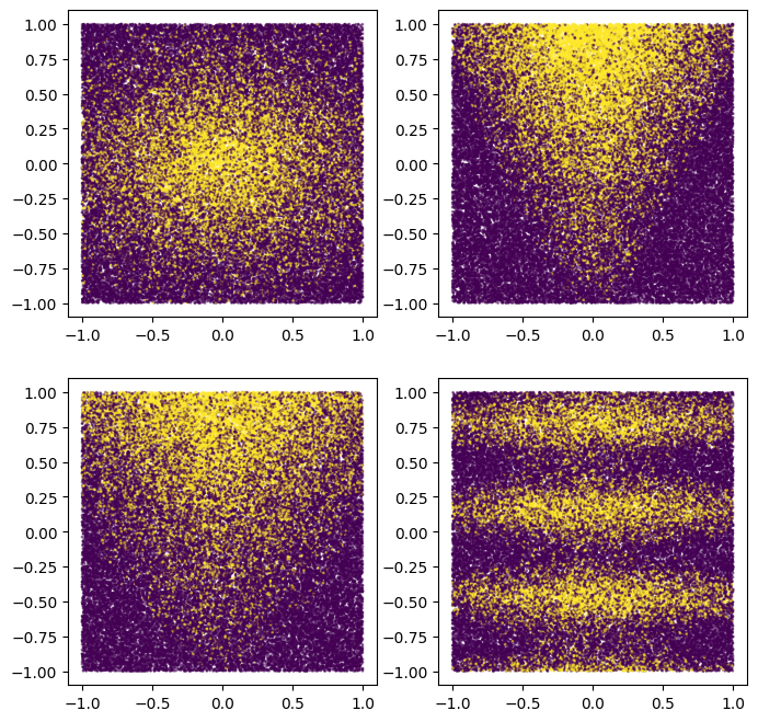
このモードはスムーズであり、軸が揃っていないことに注意してください。これはニューラルネットワークモデルに利益をもたらします。これは、ニューラルネットワークでは、デシジョンツリーよりも、円形で非整列のデシジョン境界を持つ方が簡単であるためです。

一方、2500 例の小さなデータセットでモデルをトレーニングします。これはデシジョンフォレストモデルに利益をもたらします。これは、デシジョンフォレストの方が効率的であり、利用可能なすべてのサンプル情報を活用しているためです (デシジョンフォレストは「サンプル効率的」です)。

私たちのニューラルネットワークとデシジョンフォレストアンサンブルは、両方の長所を備えています。

トレーニングとテスト用に作成しましょうtf.data.Dataset。

# 定义函数make_tf_dataset，参数为batch_size和其他参数
def make_tf_dataset(batch_size=64, **args):
  # 调用make_dataset函数，返回features和labels
  features, labels = make_dataset(**args)
  # 使用tf.data.Dataset.from_tensor_slices将features和labels转换为Dataset类型，并按batch_size划分batch
  return tf.data.Dataset.from_tensor_slices(
      (features, labels)).batch(batch_size)

# 定义变量num_features为10

# 调用make_tf_dataset函数，生成训练集train_dataset，包含2500个样本，每个样本包含num_features个特征，每个batch包含100个样本，随机数种子为1234
train_dataset = make_tf_dataset(
    num_examples=2500, num_features=num_features, batch_size=100, seed=1234)

# 调用make_tf_dataset函数，生成测试集test_dataset，包含10000个样本，每个样本包含num_features个特征，每个batch包含100个样本，随机数种子为5678
test_dataset = make_tf_dataset(
    num_examples=10000, num_features=num_features, batch_size=100, seed=5678)

モデル構造

次のようにモデル構造を定義します。

# 输入特征
raw_features = tf.keras.layers.Input(shape=(num_features,))

# 阶段1
# =======

# 公共可学习的预处理
preprocessor = tf.keras.layers.Dense(10, activation=tf.nn.relu6)
preprocess_features = preprocessor(raw_features)

# 阶段2
# =======

# 模型1：神经网络
m1_z1 = tf.keras.layers.Dense(5, activation=tf.nn.relu6)(preprocess_features)
m1_pred = tf.keras.layers.Dense(1, activation=tf.nn.sigmoid)(m1_z1)

# 模型2：神经网络
m2_z1 = tf.keras.layers.Dense(5, activation=tf.nn.relu6)(preprocess_features)
m2_pred = tf.keras.layers.Dense(1, activation=tf.nn.sigmoid)(m2_z1)


# 模型3：决策树随机森林
model_3 = tfdf.keras.RandomForestModel(num_trees=1000, random_seed=1234)
m3_pred = model_3(preprocess_features)

# 模型4：决策树随机森林
model_4 = tfdf.keras.RandomForestModel(
    num_trees=1000,
    #split_axis="SPARSE_OBLIQUE", # 取消注释此行以提高该模型的质量
    random_seed=4567)
m4_pred = model_4(preprocess_features)

# 由于TF-DF使用确定性学习算法，您应该将模型的训练种子设置为不同的值，否则两个`tfdf.keras.RandomForestModel`将完全相同。

# 阶段3
# =======

mean_nn_only = tf.reduce_mean(tf.stack([m1_pred, m2_pred], axis=0), axis=0)
mean_nn_and_df = tf.reduce_mean(
    tf.stack([m1_pred, m2_pred, m3_pred, m4_pred], axis=0), axis=0)

# Keras模型
# ============

ensemble_nn_only = tf.keras.models.Model(raw_features, mean_nn_only)
ensemble_nn_and_df = tf.keras.models.Model(raw_features, mean_nn_and_df)

Warning: The `num_threads` constructor argument is not set and the number of CPU is os.cpu_count()=32 > 32. Setting num_threads to 32. Set num_threads manually to use more than 32 cpus.


WARNING:absl:The `num_threads` constructor argument is not set and the number of CPU is os.cpu_count()=32 > 32. Setting num_threads to 32. Set num_threads manually to use more than 32 cpus.


Use /tmpfs/tmp/tmpeqn1u3t4 as temporary training directory
Warning: The model was called directly (i.e. using `model(data)` instead of using `model.predict(data)`) before being trained. The model will only return zeros until trained. The output shape might change after training Tensor("inputs:0", shape=(None, 10), dtype=float32)


WARNING:absl:The model was called directly (i.e. using `model(data)` instead of using `model.predict(data)`) before being trained. The model will only return zeros until trained. The output shape might change after training Tensor("inputs:0", shape=(None, 10), dtype=float32)


Warning: The `num_threads` constructor argument is not set and the number of CPU is os.cpu_count()=32 > 32. Setting num_threads to 32. Set num_threads manually to use more than 32 cpus.


WARNING:absl:The `num_threads` constructor argument is not set and the number of CPU is os.cpu_count()=32 > 32. Setting num_threads to 32. Set num_threads manually to use more than 32 cpus.


Use /tmpfs/tmp/tmpzrq7x74t as temporary training directory
Warning: The model was called directly (i.e. using `model(data)` instead of using `model.predict(data)`) before being trained. The model will only return zeros until trained. The output shape might change after training Tensor("inputs:0", shape=(None, 10), dtype=float32)


WARNING:absl:The model was called directly (i.e. using `model(data)` instead of using `model.predict(data)`) before being trained. The model will only return zeros until trained. The output shape might change after training Tensor("inputs:0", shape=(None, 10), dtype=float32)

モデルをトレーニングする前に、モデルをプロットして、最初のプロットと類似しているかどうかを確認できます。

# 导入plot_model函数
from keras.utils import plot_model

# 使用plot_model函数将模型ensemble_nn_and_df可视化，并保存为图片
# 参数to_file指定保存的文件路径为/tmp/model.png
# 参数show_shapes设置为True，表示在可视化图中显示每个层的输入输出形状
plot_model(ensemble_nn_and_df, to_file="/tmp/model.png", show_shapes=True)

モデルのトレーニング

前処理層と 2 つのニューラルネットワーク層は、最初にバックプロパゲーションアルゴリズムを使用してトレーニングされます。

%%time
# 编译模型
ensemble_nn_only.compile(
    optimizer=tf.keras.optimizers.Adam(),  # 使用Adam优化器来优化模型的参数
    loss=tf.keras.losses.BinaryCrossentropy(),  # 使用二元交叉熵作为损失函数
    metrics=["accuracy"]  # 使用准确率作为评估指标
)

# 训练模型
ensemble_nn_only.fit(
    train_dataset,  # 使用训练数据集进行训练
    epochs=20,  # 迭代20次
    validation_data=test_dataset  # 使用测试数据集进行验证
)

Epoch 1/20

 1/25 [>.............................] - ETA: 1:49 - loss: 0.5916 - accuracy: 0.7200
18/25 [====================>.........] - ETA: 0s - loss: 0.5695 - accuracy: 0.7556  
25/25 [==============================] - 5s 15ms/step - loss: 0.5691 - accuracy: 0.7500 - val_loss: 0.5662 - val_accuracy: 0.7392
Epoch 2/20

 1/25 [>.............................] - ETA: 0s - loss: 0.5743 - accuracy: 0.7200
19/25 [=====================>........] - ETA: 0s - loss: 0.5510 - accuracy: 0.7574
25/25 [==============================] - 0s 9ms/step - loss: 0.5542 - accuracy: 0.7500 - val_loss: 0.5554 - val_accuracy: 0.7392
Epoch 3/20

 1/25 [>.............................] - ETA: 0s - loss: 0.5623 - accuracy: 0.7200
19/25 [=====================>........] - ETA: 0s - loss: 0.5396 - accuracy: 0.7574
25/25 [==============================] - 0s 9ms/step - loss: 0.5434 - accuracy: 0.7500 - val_loss: 0.5467 - val_accuracy: 0.7392
Epoch 4/20

 1/25 [>.............................] - ETA: 0s - loss: 0.5525 - accuracy: 0.7200
17/25 [===================>..........] - ETA: 0s - loss: 0.5362 - accuracy: 0.7529
25/25 [==============================] - 0s 10ms/step - loss: 0.5342 - accuracy: 0.7500 - val_loss: 0.5384 - val_accuracy: 0.7392
Epoch 5/20

 1/25 [>.............................] - ETA: 0s - loss: 0.5433 - accuracy: 0.7200
18/25 [====================>.........] - ETA: 0s - loss: 0.5244 - accuracy: 0.7556
25/25 [==============================] - 0s 10ms/step - loss: 0.5250 - accuracy: 0.7500 - val_loss: 0.5298 - val_accuracy: 0.7392
Epoch 6/20

 1/25 [>.............................] - ETA: 0s - loss: 0.5338 - accuracy: 0.7200
18/25 [====================>.........] - ETA: 0s - loss: 0.5152 - accuracy: 0.7556
25/25 [==============================] - 0s 10ms/step - loss: 0.5154 - accuracy: 0.7500 - val_loss: 0.5205 - val_accuracy: 0.7392
Epoch 7/20

 1/25 [>.............................] - ETA: 0s - loss: 0.5241 - accuracy: 0.7200
19/25 [=====================>........] - ETA: 0s - loss: 0.5023 - accuracy: 0.7574
25/25 [==============================] - 0s 10ms/step - loss: 0.5053 - accuracy: 0.7500 - val_loss: 0.5107 - val_accuracy: 0.7392
Epoch 8/20

 1/25 [>.............................] - ETA: 0s - loss: 0.5137 - accuracy: 0.7200
19/25 [=====================>........] - ETA: 0s - loss: 0.4921 - accuracy: 0.7574
25/25 [==============================] - 0s 10ms/step - loss: 0.4947 - accuracy: 0.7500 - val_loss: 0.5007 - val_accuracy: 0.7392
Epoch 9/20

 1/25 [>.............................] - ETA: 0s - loss: 0.5029 - accuracy: 0.7200
18/25 [====================>.........] - ETA: 0s - loss: 0.4854 - accuracy: 0.7556
25/25 [==============================] - 0s 10ms/step - loss: 0.4841 - accuracy: 0.7500 - val_loss: 0.4909 - val_accuracy: 0.7392
Epoch 10/20

 1/25 [>.............................] - ETA: 0s - loss: 0.4916 - accuracy: 0.7200
19/25 [=====================>........] - ETA: 0s - loss: 0.4717 - accuracy: 0.7574
25/25 [==============================] - 0s 10ms/step - loss: 0.4738 - accuracy: 0.7500 - val_loss: 0.4815 - val_accuracy: 0.7392
Epoch 11/20

 1/25 [>.............................] - ETA: 0s - loss: 0.4799 - accuracy: 0.7200
19/25 [=====================>........] - ETA: 0s - loss: 0.4618 - accuracy: 0.7574
25/25 [==============================] - 0s 9ms/step - loss: 0.4637 - accuracy: 0.7500 - val_loss: 0.4724 - val_accuracy: 0.7392
Epoch 12/20

 1/25 [>.............................] - ETA: 0s - loss: 0.4680 - accuracy: 0.7200
19/25 [=====================>........] - ETA: 0s - loss: 0.4522 - accuracy: 0.7574
25/25 [==============================] - 0s 9ms/step - loss: 0.4541 - accuracy: 0.7500 - val_loss: 0.4639 - val_accuracy: 0.7392
Epoch 13/20

 1/25 [>.............................] - ETA: 0s - loss: 0.4559 - accuracy: 0.7200
18/25 [====================>.........] - ETA: 0s - loss: 0.4473 - accuracy: 0.7556
25/25 [==============================] - 0s 9ms/step - loss: 0.4453 - accuracy: 0.7500 - val_loss: 0.4561 - val_accuracy: 0.7392
Epoch 14/20

 1/25 [>.............................] - ETA: 0s - loss: 0.4441 - accuracy: 0.7200
18/25 [====================>.........] - ETA: 0s - loss: 0.4392 - accuracy: 0.7556
25/25 [==============================] - 0s 9ms/step - loss: 0.4373 - accuracy: 0.7500 - val_loss: 0.4491 - val_accuracy: 0.7398
Epoch 15/20

 1/25 [>.............................] - ETA: 0s - loss: 0.4332 - accuracy: 0.7300
19/25 [=====================>........] - ETA: 0s - loss: 0.4280 - accuracy: 0.7621
25/25 [==============================] - 0s 10ms/step - loss: 0.4300 - accuracy: 0.7552 - val_loss: 0.4426 - val_accuracy: 0.7439
Epoch 16/20

 1/25 [>.............................] - ETA: 0s - loss: 0.4227 - accuracy: 0.7300
18/25 [====================>.........] - ETA: 0s - loss: 0.4252 - accuracy: 0.7667
25/25 [==============================] - 0s 10ms/step - loss: 0.4234 - accuracy: 0.7624 - val_loss: 0.4366 - val_accuracy: 0.7508
Epoch 17/20

 1/25 [>.............................] - ETA: 0s - loss: 0.4132 - accuracy: 0.7400
19/25 [=====================>........] - ETA: 0s - loss: 0.4153 - accuracy: 0.7753
25/25 [==============================] - 0s 9ms/step - loss: 0.4173 - accuracy: 0.7692 - val_loss: 0.4310 - val_accuracy: 0.7608
Epoch 18/20

 1/25 [>.............................] - ETA: 0s - loss: 0.4047 - accuracy: 0.7500
19/25 [=====================>........] - ETA: 0s - loss: 0.4095 - accuracy: 0.7800
25/25 [==============================] - 0s 9ms/step - loss: 0.4115 - accuracy: 0.7764 - val_loss: 0.4255 - val_accuracy: 0.7752
Epoch 19/20

 1/25 [>.............................] - ETA: 0s - loss: 0.3966 - accuracy: 0.7600
18/25 [====================>.........] - ETA: 0s - loss: 0.4076 - accuracy: 0.7922
25/25 [==============================] - 0s 10ms/step - loss: 0.4059 - accuracy: 0.7880 - val_loss: 0.4201 - val_accuracy: 0.7847
Epoch 20/20

 1/25 [>.............................] - ETA: 0s - loss: 0.3887 - accuracy: 0.7900
19/25 [=====================>........] - ETA: 0s - loss: 0.3981 - accuracy: 0.8053
25/25 [==============================] - 0s 9ms/step - loss: 0.4003 - accuracy: 0.7988 - val_loss: 0.4148 - val_accuracy: 0.7913
CPU times: user 8.67 s, sys: 1.46 s, total: 10.1 s
Wall time: 9.49 s





<keras.src.callbacks.History at 0x7fac640c79a0>

前処理と 2 つのニューラルネットワーク部分のみを含めてこれを評価してみましょう。

# 评估神经网络模型（仅使用NN #1和NN #2）
evaluation_nn_only = ensemble_nn_only.evaluate(test_dataset, return_dict=True)

# 打印准确率（仅使用NN #1和NN #2）
print("Accuracy (NN #1 and #2 only): ", evaluation_nn_only["accuracy"])

# 打印损失值（仅使用NN #1和NN #2）
print("Loss (NN #1 and #2 only): ", evaluation_nn_only["loss"])

  1/100 [..............................] - ETA: 0s - loss: 0.3536 - accuracy: 0.8400
 30/100 [========>.....................] - ETA: 0s - loss: 0.4103 - accuracy: 0.7967
 59/100 [================>.............] - ETA: 0s - loss: 0.4093 - accuracy: 0.7920
 88/100 [=========================>....] - ETA: 0s - loss: 0.4119 - accuracy: 0.7917
100/100 [==============================] - 0s 2ms/step - loss: 0.4148 - accuracy: 0.7913
Accuracy (NN #1 and #2 only):  0.7912999987602234
Loss (NN #1 and #2 only):  0.4147580564022064

2 つのデシジョンフォレストコンポーネントを順番にトレーニングしてみましょう。

# 对训练数据集进行预处理
# 使用map函数对train_dataset中的每个样本进行预处理，preprocessor函数用于对样本进行处理
# 返回的结果是一个新的数据集train_dataset_with_preprocessing，其中每个样本都经过了预处理
train_dataset_with_preprocessing = train_dataset.map(lambda x,y: (preprocessor(x), y))

# 对测试数据集进行预处理
# 使用map函数对test_dataset中的每个样本进行预处理，preprocessor函数用于对样本进行处理
# 返回的结果是一个新的数据集test_dataset_with_preprocessing，其中每个样本都经过了预处理
test_dataset_with_preprocessing = test_dataset.map(lambda x,y: (preprocessor(x), y))

# 使用model_3对预处理后的训练数据集进行训练
model_3.fit(train_dataset_with_preprocessing)

# 使用model_4对预处理后的训练数据集进行训练
model_4.fit(train_dataset_with_preprocessing)

WARNING:tensorflow:AutoGraph could not transform <function <lambda> at 0x7fad5d4b6700> and will run it as-is.
Cause: could not parse the source code of <function <lambda> at 0x7fad5d4b6700>: no matching AST found among candidates:

To silence this warning, decorate the function with @tf.autograph.experimental.do_not_convert


WARNING:tensorflow:AutoGraph could not transform <function <lambda> at 0x7fad5d4b6700> and will run it as-is.
Cause: could not parse the source code of <function <lambda> at 0x7fad5d4b6700>: no matching AST found among candidates:

To silence this warning, decorate the function with @tf.autograph.experimental.do_not_convert


WARNING: AutoGraph could not transform <function <lambda> at 0x7fad5d4b6700> and will run it as-is.
Cause: could not parse the source code of <function <lambda> at 0x7fad5d4b6700>: no matching AST found among candidates:

To silence this warning, decorate the function with @tf.autograph.experimental.do_not_convert
WARNING:tensorflow:AutoGraph could not transform <function <lambda> at 0x7facb40f80d0> and will run it as-is.
Cause: could not parse the source code of <function <lambda> at 0x7facb40f80d0>: no matching AST found among candidates:

To silence this warning, decorate the function with @tf.autograph.experimental.do_not_convert


WARNING:tensorflow:AutoGraph could not transform <function <lambda> at 0x7facb40f80d0> and will run it as-is.
Cause: could not parse the source code of <function <lambda> at 0x7facb40f80d0>: no matching AST found among candidates:

To silence this warning, decorate the function with @tf.autograph.experimental.do_not_convert


WARNING: AutoGraph could not transform <function <lambda> at 0x7facb40f80d0> and will run it as-is.
Cause: could not parse the source code of <function <lambda> at 0x7facb40f80d0>: no matching AST found among candidates:

To silence this warning, decorate the function with @tf.autograph.experimental.do_not_convert
Reading training dataset...
Training dataset read in 0:00:03.527053. Found 2500 examples.
Training model...


[INFO 23-07-10 11:10:25.0183 UTC kernel.cc:1243] Loading model from path /tmpfs/tmp/tmpeqn1u3t4/model/ with prefix 03256340d0ca40b0


Model trained in 0:00:01.894803
Compiling model...


[INFO 23-07-10 11:10:25.9915 UTC decision_forest.cc:660] Model loaded with 1000 root(s), 314626 node(s), and 10 input feature(s).
[INFO 23-07-10 11:10:25.9915 UTC abstract_model.cc:1311] Engine "RandomForestOptPred" built
[INFO 23-07-10 11:10:25.9916 UTC kernel.cc:1075] Use fast generic engine


WARNING:tensorflow:AutoGraph could not transform <function simple_ml_inference_op_with_handle at 0x7fac685de700> and will run it as-is.
Please report this to the TensorFlow team. When filing the bug, set the verbosity to 10 (on Linux, `export AUTOGRAPH_VERBOSITY=10`) and attach the full output.
Cause: could not get source code
To silence this warning, decorate the function with @tf.autograph.experimental.do_not_convert


WARNING:tensorflow:AutoGraph could not transform <function simple_ml_inference_op_with_handle at 0x7fac685de700> and will run it as-is.
Please report this to the TensorFlow team. When filing the bug, set the verbosity to 10 (on Linux, `export AUTOGRAPH_VERBOSITY=10`) and attach the full output.
Cause: could not get source code
To silence this warning, decorate the function with @tf.autograph.experimental.do_not_convert


WARNING: AutoGraph could not transform <function simple_ml_inference_op_with_handle at 0x7fac685de700> and will run it as-is.
Please report this to the TensorFlow team. When filing the bug, set the verbosity to 10 (on Linux, `export AUTOGRAPH_VERBOSITY=10`) and attach the full output.
Cause: could not get source code
To silence this warning, decorate the function with @tf.autograph.experimental.do_not_convert
Model compiled.
Reading training dataset...
Training dataset read in 0:00:00.210194. Found 2500 examples.
Training model...


[INFO 23-07-10 11:10:28.3455 UTC kernel.cc:1243] Loading model from path /tmpfs/tmp/tmpzrq7x74t/model/ with prefix a093792264d04fac


Model trained in 0:00:01.800354
Compiling model...


[INFO 23-07-10 11:10:29.2816 UTC decision_forest.cc:660] Model loaded with 1000 root(s), 316314 node(s), and 10 input feature(s).
[INFO 23-07-10 11:10:29.2816 UTC kernel.cc:1075] Use fast generic engine


Model compiled.
CPU times: user 20.1 s, sys: 1.49 s, total: 21.6 s
Wall time: 8.92 s





<keras.src.callbacks.History at 0x7fac5073e430>

デシジョンフォレストの評価

決定の森を 1 つずつ評価してみましょう。

# 给模型添加评估指标
model_3.compile(["accuracy"])
model_4.compile(["accuracy"])

# 使用预处理后的测试数据对模型3进行评估，并返回评估结果的字典形式
evaluation_df3_only = model_3.evaluate(test_dataset_with_preprocessing, return_dict=True)

# 使用预处理后的测试数据对模型4进行评估，并返回评估结果的字典形式
evaluation_df4_only = model_4.evaluate(test_dataset_with_preprocessing, return_dict=True)

# 打印模型3的准确率评估结果
print("Accuracy (DF #3 only): ", evaluation_df3_only["accuracy"])

# 打印模型4的准确率评估结果
print("Accuracy (DF #4 only): ", evaluation_df4_only["accuracy"])

  1/100 [..............................] - ETA: 29s - loss: 0.0000e+00 - accuracy: 0.8600
  6/100 [>.............................] - ETA: 0s - loss: 0.0000e+00 - accuracy: 0.8200 
 12/100 [==>...........................] - ETA: 0s - loss: 0.0000e+00 - accuracy: 0.8300
 17/100 [====>.........................] - ETA: 0s - loss: 0.0000e+00 - accuracy: 0.8218
 22/100 [=====>........................] - ETA: 0s - loss: 0.0000e+00 - accuracy: 0.8173
 28/100 [=======>......................] - ETA: 0s - loss: 0.0000e+00 - accuracy: 0.8129
 34/100 [=========>....................] - ETA: 0s - loss: 0.0000e+00 - accuracy: 0.8124
 40/100 [===========>..................] - ETA: 0s - loss: 0.0000e+00 - accuracy: 0.8138
 46/100 [============>.................] - ETA: 0s - loss: 0.0000e+00 - accuracy: 0.8161
 52/100 [==============>...............] - ETA: 0s - loss: 0.0000e+00 - accuracy: 0.8173
 58/100 [================>.............] - ETA: 0s - loss: 0.0000e+00 - accuracy: 0.8178
 64/100 [==================>...........] - ETA: 0s - loss: 0.0000e+00 - accuracy: 0.8156
 69/100 [===================>..........] - ETA: 0s - loss: 0.0000e+00 - accuracy: 0.8165
 75/100 [=====================>........] - ETA: 0s - loss: 0.0000e+00 - accuracy: 0.8175
 80/100 [=======================>......] - ETA: 0s - loss: 0.0000e+00 - accuracy: 0.8166
 86/100 [========================>.....] - ETA: 0s - loss: 0.0000e+00 - accuracy: 0.8166
 92/100 [==========================>...] - ETA: 0s - loss: 0.0000e+00 - accuracy: 0.8153
 98/100 [============================>.] - ETA: 0s - loss: 0.0000e+00 - accuracy: 0.8152
100/100 [==============================] - 1s 10ms/step - loss: 0.0000e+00 - accuracy: 0.8150

  1/100 [..............................] - ETA: 12s - loss: 0.0000e+00 - accuracy: 0.8500
  6/100 [>.............................] - ETA: 0s - loss: 0.0000e+00 - accuracy: 0.8250 
 12/100 [==>...........................] - ETA: 0s - loss: 0.0000e+00 - accuracy: 0.8325
 18/100 [====>.........................] - ETA: 0s - loss: 0.0000e+00 - accuracy: 0.8228
 24/100 [======>.......................] - ETA: 0s - loss: 0.0000e+00 - accuracy: 0.8158
 30/100 [========>.....................] - ETA: 0s - loss: 0.0000e+00 - accuracy: 0.8127
 36/100 [=========>....................] - ETA: 0s - loss: 0.0000e+00 - accuracy: 0.8122
 42/100 [===========>..................] - ETA: 0s - loss: 0.0000e+00 - accuracy: 0.8148
 48/100 [=============>................] - ETA: 0s - loss: 0.0000e+00 - accuracy: 0.8144
 54/100 [===============>..............] - ETA: 0s - loss: 0.0000e+00 - accuracy: 0.8176
 60/100 [=================>............] - ETA: 0s - loss: 0.0000e+00 - accuracy: 0.8153
 66/100 [==================>...........] - ETA: 0s - loss: 0.0000e+00 - accuracy: 0.8150
 71/100 [====================>.........] - ETA: 0s - loss: 0.0000e+00 - accuracy: 0.8169
 76/100 [=====================>........] - ETA: 0s - loss: 0.0000e+00 - accuracy: 0.8176
 81/100 [=======================>......] - ETA: 0s - loss: 0.0000e+00 - accuracy: 0.8167
 86/100 [========================>.....] - ETA: 0s - loss: 0.0000e+00 - accuracy: 0.8162
 91/100 [==========================>...] - ETA: 0s - loss: 0.0000e+00 - accuracy: 0.8149
 96/100 [===========================>..] - ETA: 0s - loss: 0.0000e+00 - accuracy: 0.8147
100/100 [==============================] - 1s 10ms/step - loss: 0.0000e+00 - accuracy: 0.8149
Accuracy (DF #3 only):  0.8149999976158142
Accuracy (DF #4 only):  0.8148999810218811

モデルポートフォリオ全体を評価してみましょう。

# 编译模型
ensemble_nn_and_df.compile(
    loss=tf.keras.losses.BinaryCrossentropy(), metrics=["accuracy"])

# 评估模型
evaluation_nn_and_df = ensemble_nn_and_df.evaluate(
    test_dataset, return_dict=True)

# 打印准确率和损失值
print("Accuracy (2xNN and 2xDF): ", evaluation_nn_and_df["accuracy"])
print("Loss (2xNN and 2xDF): ", evaluation_nn_and_df["loss"])

  1/100 [..............................] - ETA: 23s - loss: 0.3324 - accuracy: 0.8600
  6/100 [>.............................] - ETA: 0s - loss: 0.3850 - accuracy: 0.8267 
 12/100 [==>...........................] - ETA: 0s - loss: 0.3650 - accuracy: 0.8317
 18/100 [====>.........................] - ETA: 0s - loss: 0.3679 - accuracy: 0.8261
 24/100 [======>.......................] - ETA: 0s - loss: 0.3723 - accuracy: 0.8229
 30/100 [========>.....................] - ETA: 0s - loss: 0.3752 - accuracy: 0.8200
 35/100 [=========>....................] - ETA: 0s - loss: 0.3742 - accuracy: 0.8200
 40/100 [===========>..................] - ETA: 0s - loss: 0.3736 - accuracy: 0.8198
 46/100 [============>.................] - ETA: 0s - loss: 0.3723 - accuracy: 0.8207
 52/100 [==============>...............] - ETA: 0s - loss: 0.3716 - accuracy: 0.8213
 58/100 [================>.............] - ETA: 0s - loss: 0.3722 - accuracy: 0.8193
 64/100 [==================>...........] - ETA: 0s - loss: 0.3754 - accuracy: 0.8178
 70/100 [====================>.........] - ETA: 0s - loss: 0.3745 - accuracy: 0.8184
 76/100 [=====================>........] - ETA: 0s - loss: 0.3753 - accuracy: 0.8170
 82/100 [=======================>......] - ETA: 0s - loss: 0.3757 - accuracy: 0.8151
 88/100 [=========================>....] - ETA: 0s - loss: 0.3760 - accuracy: 0.8147
 94/100 [===========================>..] - ETA: 0s - loss: 0.3785 - accuracy: 0.8130
100/100 [==============================] - ETA: 0s - loss: 0.3795 - accuracy: 0.8133
100/100 [==============================] - 1s 10ms/step - loss: 0.3795 - accuracy: 0.8133
Accuracy (2xNN and 2xDF):  0.8133000135421753
Loss (2xNN and 2xDF):  0.37953513860702515

作業を完了するには、ニューラルネットワーク層をもう少し微調整しましょう。DF モデルは事前トレーニング済みの埋め込みに依存しているため、事前トレーニング済みの埋め込みを微調整しないことに注意してください (後で再トレーニングしない限り)。

要約すると、次のようになります。

# 输出NN #1和#2的准确率
print(f"Accuracy (NN #1 and #2 only):\t{
      
      evaluation_nn_only['accuracy']:.6f}")
# 输出DF #3的准确率
print(f"Accuracy (DF #3 only):\t\t{
      
      evaluation_df3_only['accuracy']:.6f}")
# 输出DF #4的准确率
print(f"Accuracy (DF #4 only):\t\t{
      
      evaluation_df4_only['accuracy']:.6f}")
# 输出分割线
print("----------------------------------------")
# 输出2xNN和2xDF的准确率
print(f"Accuracy (2xNN and 2xDF):\t{
      
      evaluation_nn_and_df['accuracy']:.6f}")

# 定义一个函数，计算准确率的增长百分比
def delta_percent(src_eval, key):
  # 获取源准确率
  src_acc = src_eval["accuracy"]
  # 获取最终准确率
  final_acc = evaluation_nn_and_df["accuracy"]
  # 计算准确率的增长
  increase = final_acc - src_acc
  # 输出增长百分比
  print(f"\t\t\t\t  {
      
      increase:+.6f} over {
      
      key}")

# 分别计算NN #1和#2、DF #3、DF #4的准确率增长百分比
delta_percent(evaluation_nn_only, "NN #1 and #2 only")
delta_percent(evaluation_df3_only, "DF #3 only")
delta_percent(evaluation_df4_only, "DF #4 only")

Accuracy (NN #1 and #2 only):	0.791300
Accuracy (DF #3 only):		0.815000
Accuracy (DF #4 only):		0.814900
----------------------------------------
Accuracy (2xNN and 2xDF):	0.813300
				  +0.022000 over NN #1 and #2 only
				  -0.001700 over DF #3 only
				  -0.001600 over DF #4 only

ここでは、結合されたモデルが個々の部分よりも優れていることがわかります。これが、統合されたアプローチが非常にうまく機能する理由です。

次は何ですか？

この例では、デシジョンフォレストとニューラルネットワークを組み合わせる方法を説明しました。ニューラルネットワークとデシジョンフォレストをさらにトレーニングするための追加のステップ。

さらに、明確にするために、デシジョンフォレストは前処理された入力のみを受け取ります。ただし、デシジョンフォレストは多くの場合、生データの利用に非常に優れています。元の特徴をデシジョンフォレストモデルにフィードすることによって、モデルを改善することもできます。

この例では、最終モデルは個々のモデル予測の平均です。すべてのモデルのパフォーマンスが同様であれば、このソリューションはうまく機能します。ただし、サブモデルの 1 つが非常に優れている場合、それを他のモデルと集約することは実際には有害である可能性があります (またはその逆も同様です。たとえば、例の数を 1k に減らして、それがニューラルネットワークにどのように深刻な影響を与えるかを確認してください。または2 番目にランダムフォレストモデルで「SPARSE_OBLIQUE」分割を有効にします)。