Matriz de transformación de puntos en sistema de coordenadas 2D (traslación, escalado, rotación, corte incorrecto)

1. Traducción

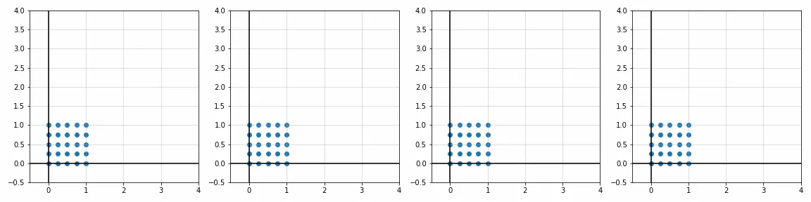
En el espacio 2D, a menudo necesitamos trasladar un punto a otro. Supongamos un punto P ( x , y ) P(x,y) en el espacio$P(x,y)$ ; dirígelo a$x,$Traducirtx t_x$en\; la\; dirección\; y$$t_{}$，$t_{}$, suponiendo que las coordenadas del punto después de la traslación son $(x^{\prime },y^{\prime })$, entonces la operación de traducción de los puntos anteriores se puede resumir en la siguiente fórmula:
$$\begin{array}{rl}& X^{\prime }=X+t_{}\\ & y^{\prime }=X+t_{}\end{array}$$
Usando una matriz homogénea se expresa de la siguiente manera:
$$\left[\begin{array}{c}{X}^{\prime }\\ y^{\prime }\\ \end{array}\right]=\left[\begin{array}{ccc}1& b& t_{}\\ 0& 1& t_{}\\ & & \end{array}\right]\left[\begin{array}{c}X\\ y\\ \end{array}\right]$$

import numpy as np


def translation():
    """
    原始数组a 三个点(1,1) (4,4) (7,7)
    构建齐次矩阵 P
    构建变换矩阵 T
    """
    a = np.array([[1, 1],
               [4, 4],
               [7, 7]])

    P = np.array([a[:, 0],
               a[:, 1],
               np.ones(len(a))])

    T = np.array([[1, 0, 2],
               [0, 1, 2],
               [0, 0, 1]])
    return np.dot(T, P)


print(translation())

"""
[[3. 6. 9.]
 [3. 6. 9.]
 [1. 1. 1.]]
"""

Demostración del efecto de animación

import matplotlib
import matplotlib.pyplot as plt
import numpy as np

X, Y = np.mgrid[0:1:5j, 0:1:5j]
x, y = X.ravel(), Y.ravel()

def trans_translate(x, y, tx, ty):
    T = [[1, 0, tx],
         [0, 1, ty],
         [0, 0, 1]]
    T = np.array(T)
    P = np.array([x, y, [1] * x.size])
    return np.dot(T, P)

fig, ax = plt.subplots(1, 4)
T_ = [[0, 0], [2.3, 0], [0, 1.7], [2, 2]]
for i in range(4):
    tx, ty = T_[i]
    x_, y_, _ = trans_translate(x, y, tx, ty)
    ax[i].scatter(x_, y_)
    ax[i].set_title(r'$t_x={0:.2f}$ , $t_y={1:.2f}$'.format(tx, ty))

    ax[i].set_xlim([-0.5, 4])
    ax[i].set_ylim([-0.5, 4])
    ax[i].grid(alpha=0.5)
    ax[i].axhline(y=0, color='k')
    ax[i].axvline(x=0, color='k')
plt.show()

2. Escalado

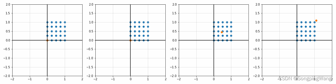
En el espacio 2D, un punto $(X,y)$ relativo a otro punto$({pag}_{},{pag}_{})$ para la operación de escala, también podríamos escalar el factor en$Las\; direcciones\; xey$ son respectivamente:$s_{},s_{}$, entonces la operación de escala anterior se puede resumir como la siguiente fórmula:
$$\begin{array}{rlr}& X^{\prime }=s_{}(x-{pag}_{})+{pag}_{}& =s_{}X+{pag}_{}(1-s_{})\\ & y^{\prime }=s_{}(y-{pag}_{})+{pag}_{}& =s_{}y+{pag}_{}(1-s_{}\end{array}$$
Usando una matriz homogénea se expresa de la siguiente manera:
$$\left[\begin{array}{c}{X}^{\prime }\\ y^{\prime }\\ \end{array}\right]=\left[\begin{array}{ccc}{s}_{}& 0& {pag}_{}(1-s_{})\\ 0& s_{}& {pag}_{}(1-s_{})\\ & & \end{array}\right]\left[\begin{array}{c}X\\ y\\ \end{array}\right]$$

def trans_scale(x, y, px, py, sx, sy):
    T = [[sx, 0 , px*(1 - sx)],
         [0 , sy, py*(1 - sy)],
         [0 , 0 , 1          ]]
    T = np.array(T)
    P = np.array([x, y, [1]*x.size])
    return np.dot(T, P)

fig, ax = plt.subplots(1, 4)
S_ = [[1, 1], [1.8, 1], [1, 1.7], [2, 2]]
P_ = [[0, 0], [0, 0], [0.45, 0.45], [1.1, 1.1]]
for i in range(4):
    sx, sy = S_[i]; px, py = P_[i]
    x_, y_, _ = trans_scale(x, y, px, py, sx, sy)
    ax[i].scatter(x_, y_)
    ax[i].scatter(px, py)
    ax[i].set_title(r'$p_x={0:.2f}$ , $p_y={1:.2f}$'.format(px, py) + '\n'
                    r'$s_x={0:.2f}$ , $s_y={1:.2f}$'.format(sx, sy))
    
    ax[i].set_xlim([-2, 2])
    ax[i].set_ylim([-2, 2])
    ax[i].grid(alpha=0.5)
    ax[i].axhline(y=0, color='k')
    ax[i].axvline(x=0, color='k')

plt.show()

3. Rotación

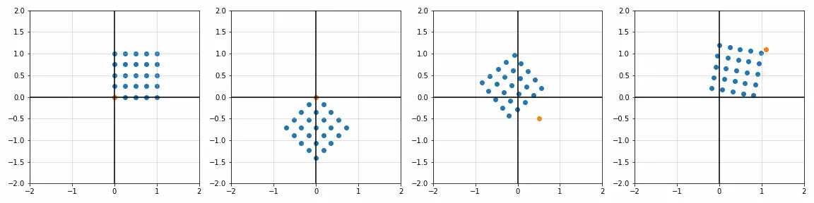
En el espacio 2D, para un punto $(X,y)$ relativo a otro punto$({pag}_{},{pag}_{})$ para la operación de rotación, generalmente el sentido antihorario es positivo y el sentido horario es negativo, asumiendo que el ángulo de rotación es$\beta$ , entonces los puntos anteriores$x,y$ relativo al punto${pag}_{},{pag}_{}$El ángulo de rotación $Defina\; la\; función\; \beta$ como una función:
$$\left[\begin{array}{c}{X}^{\prime }\\ y^{\prime }\\ \end{array}\right]=\left[\begin{array}{ccc}\mathrm{porque}b& -\mathrm{pecado}b& {pag}_{}(1-\mathrm{porque}segundo)+{pag}_{}\mathrm{pecado}b\\ \mathrm{pecado}b& \mathrm{porque}b& {pag}_{}(1-\mathrm{porque}segundo)+{pag}_{}\mathrm{pecado}b\\ & & \end{array}\right]\left[\begin{array}{c}X\\ y\\ \end{array}\right]$$

def trans_rotate(x, y, px, py, beta):
    beta = np.deg2rad(beta)
    T = [[np.cos(beta), -np.sin(beta), px*(1 - np.cos(beta)) + py*np.sin(beta)],
         [np.sin(beta),  np.cos(beta), py*(1 - np.cos(beta)) - px*np.sin(beta)],
         [0           ,  0           , 1                                      ]]
    T = np.array(T)
    P = np.array([x, y, [1]*x.size])
    return np.dot(T, P)

fig, ax = plt.subplots(1, 4)

R_ = [0, 225, 40, -10]
P_ = [[0, 0], [0, 0], [0.5, -0.5], [1.1, 1.1]]

for i in range(4):
    beta = R_[i]; px, py = P_[i]
    x_, y_, _ = trans_rotate(x, y, px, py, beta)
    ax[i].scatter(x_, y_)
    ax[i].scatter(px, py)
    ax[i].set_title(r'$\beta={0}°$ , $p_x={1:.2f}$ , $p_y={2:.2f}$'.format(beta, px, py))
    
    ax[i].set_xlim([-2, 2])
    ax[i].set_ylim([-2, 2])
    ax[i].grid(alpha=0.5)
    ax[i].axhline(y=0, color='k')
    ax[i].axvline(x=0, color='k')

plt.show（）

4. esquila

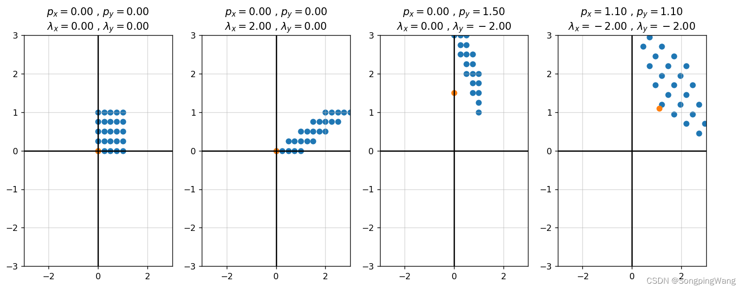
En el espacio 2D, para un punto $(X,y)$ relativo a otro punto$({pag}_{},{pag}_{})$ para operaciones de corte incorrecto, que generalmente se utiliza para el procesamiento de deformación de objetos elásticos. Supongamos que los parámetros de corte incorrecto a lo largo de las direcciones x e y son${yo}_{},{yo}_{}$, entonces la operación de corte incorrecto se puede resumir y expresar como una matriz homogénea de la siguiente manera:

$$\left[\begin{array}{c}{X}^{\prime }\\ y^{\prime }\\ \end{array}\right]=\left[\begin{array}{ccc}1& {yo}_{}& -{yo}_{}{pag}_{}\\ {yo}_{}& 1& -{yo}_{}{pag}_{}\\ & & \end{array}\right]\left[\begin{array}{c}X\\ y\\ \end{array}\right]$$

import matplotlib.pyplot as plt
import numpy as np


X, Y = np.mgrid[0:1:5j, 0:1:5j]
x, y = X.ravel(), Y.ravel()

def trans_shear(x, y, px, py, lambdax, lambday):
    T = [[1      , lambdax, -lambdax*px],
         [lambday, 1      , -lambday*py],
         [0      , 0      ,  1         ]]
    T = np.array(T)
    P = np.array([x, y, [1]*x.size])
    return np.dot(T, P)

fig, ax = plt.subplots(1, 4)

L_ = [[0, 0], [2, 0], [0, -2], [-2, -2]]
P_ = [[0, 0], [0, 0], [0, 1.5], [1.1, 1.1]]

for i in range(4):
    lambdax, lambday = L_[i]; px, py = P_[i]
    x_, y_, _ = trans_shear(x, y, px, py, lambdax, lambday)
    ax[i].scatter(x_, y_)
    ax[i].scatter(px, py)
    ax[i].set_title(r'$p_x={0:.2f}$ , $p_y={1:.2f}$'.format(px, py) + '\n'
                    r'$\lambda_x={0:.2f}$ , $\lambda_y={1:.2f}$'.format(lambdax, lambday))

    ax[i].set_xlim([-3, 3])
    ax[i].set_ylim([-3, 3])
    ax[i].grid(alpha=0.5)
    ax[i].axhline(y=0, color='k')
    ax[i].axvline(x=0, color='k')

plt.show()

5. Reflexión

Para reflejar, el vector normal v del eje de simetría $v(v_{},v_{})$ , la matriz espejo$t_{}$Ejemplo:
$$\left[\begin{array}{ccc}1-2x{\_}_{}{}^2& -2x\_{\_}_{}{y}_{}& 0\\ -2x\_{\_}_{}{y}_{}& 1-2{años}_{}{}^2& 0\\ & & \end{array}\right]$$
Además, se necesita un punto para representar la posición del eje de simetría (cualquier punto entre los 2 puntos del eje de simetría), expresado como $METRO\left(x_{},y_{}\right)$ , matriz de transformación$h=t_{}\ast t_{}\ast t_t^{-}$:
$$h=\left[\begin{array}{ccc}1& 0& 0\\ 0& 1& 0\\ X_{}& y_{}& \end{array}\right]\left[\begin{array}{ccc}1-2x{\_}_{}{}^2& -2x\_{\_}_{}{y}_{}& 0\\ -2x\_{\_}_{}{y}_{}& 1-2{años}_{}{}^2& 0\\ & & \end{array}\right]\left[\begin{array}{ccc}1& 0& 0\\ 0& 1& 0\\ -x{\_}_{}& -y_{}& \end{array}\right]$$
Las coordenadas después de la duplicación son $t_{}\ast t_{}\ast t_{}\ast t_t^{-}$。

Matriz de espejo para reflejar a lo largo del eje X
$$\left[\begin{array}{ccc}1& 0& 0\\ 0& -1& 0\\ & & \end{array}\right]$$
Matriz de espejo para reflejar a lo largo del
$$\left[\begin{array}{ccc}-1& 0& 0\\ 0& 1& 0\\ & & \end{array}\right]$$

import numpy as np


a = np.array([[1, 2],
              [2, 2],
              [3, 5],
              [4, 6]])
a = np.array([a[:,0], a[:,1], np.ones(len(a))])
print("\n",a)
print("--------------------------------")

T_x = np.array( [[ 1,  0,  0],
                 [ 0, -1,  0],
                 [ 1,  0,  1]])
print("\n",np.dot(T_x, a))
print("=================================")
T_y = np.array( [[-1,  0,  0],
                 [ 0,  1,  0],
                 [ 0,  1,  1]])
print("\n",np.dot(T_y, a))

Referencia:
https://zhuanlan.zhihu.com/p/387578291
https://zhuanlan.zhihu.com/p/187411029
https://blog.csdn.net/Akiyama_sou/article/details/122144415