Vi que 阿昆的科研日常escribí un artículo sobre cómo ocultar el eje sin ocultar la escala. Usé el objeto Axle en XRuler para implementarlo, pero lo probé. No está disponible directamente en la versión R2023A. Lo resolví y hablé sobre estas cosas interesantes al mismo tiempo objetos ocultos y sus otros usos.


1 Ocultar líneas de marco de eje
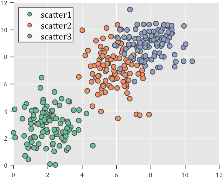
Supongamos que escribimos el siguiente código:
rng(12)
% 生成随机点
mu = [2 3; 6 7; 8 9];
S  = cat(3,[1 0; 0 2],[1 0; 0 2],[1 0; 0 1]);
r1 = abs(mvnrnd(mu(1,:),S(:,:,1),100));
r2 = abs(mvnrnd(mu(2,:),S(:,:,2),100));
r3 = abs(mvnrnd(mu(3,:),S(:,:,3),100));
% 绘制散点图
hold on
propCell={

    'LineWidth',1.2,'MarkerEdgeColor',[.3,.3,.3],'SizeData',60};
scatter(r1(:,1),r1(:,2),'filled','CData',[0.40 0.76 0.60],propCell{

    :});
scatter(r2(:,1),r2(:,2),'filled','CData',[0.99 0.55 0.38],propCell{

    :});
scatter(r3(:,1),r3(:,2),'filled','CData',[0.55 0.63 0.80],propCell{

    :});
% 增添图例
lgd=legend('scatter1','scatter2','scatter3');
lgd.Location='northwest';
lgd.FontSize=14;
% 半透明图例
pause(1e-6)
lgd.BoxFace.ColorType='truecoloralpha';
lgd.BoxFace.ColorData=uint8(255*[1;1;1;.8]);
% 坐标区域基础修饰
ax=gca; grid on
ax.FontName   = 'Cambria';
ax.Color      = [0.9,0.9,0.9];
ax.Box        = 'off';
ax.TickDir    = 'out';
ax.GridColor  = [1 1 1];
ax.GridAlpha  = 1;
ax.LineWidth  = 1;
ax.XColor     = [0.2,0.2,0.2];
ax.YColor     = [0.2,0.2,0.2];
ax.TickLength = [0.015 0.025];

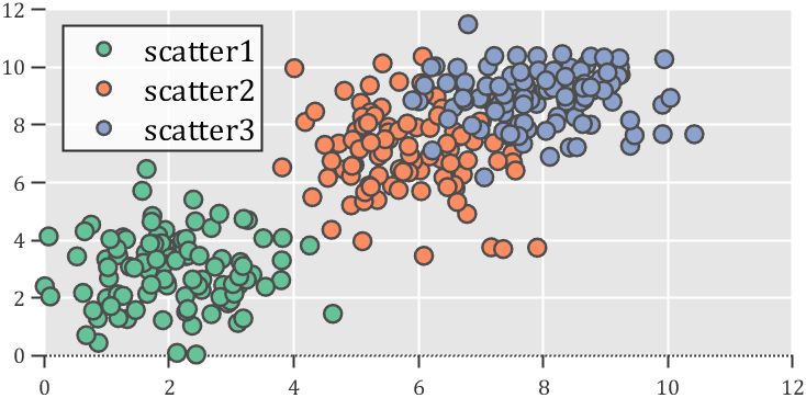
Agregue el siguiente código al final del código para ocultar el eje:
% 隐藏轴线
ax=gca;
pause(1e-6)
ax.XRuler.Axle.LineStyle='none';
ax.YRuler.Axle.LineStyle='none';

Tenga en cuenta que para la versión más nueva, Axle no se mostrará directamente como un subobjeto de XRuler. Toma una pausa por un tiempo antes de que el objeto se genere y se agregue como un subobjeto de XRuler. Esto es diferente de la versión anterior. . Por supuesto, sin configurar el formato de línea, también es una forma de ajustar directamente su visibilidad a no:
% 隐藏轴线
ax=gca;
pause(1e-6)
ax.XRuler.Axle.Visible='off';
ax.YRuler.Axle.Visible='off';
Y si configura el formato de línea, no solo puede establecerlo en 'ninguno', sino también en 'sólido' | 'discontinuo' | 'punteado' | 'guionado' | 'ninguno' y otros tipos (tenga en cuenta la x- eje en la figura siguiente)


2 ejes logarítmicos
En general, las siguientes funciones se pueden usar para dibujar un gráfico de eje logarítmico, pero todos los gráficos se dibujan como gráficos de líneas:
- gráfica de escala logarítmica doble loglog
- semilogx gráfico semi-logarítmico (el eje x tiene escala logarítmica)
- gráfica semilogarítmica de semilogía (el eje y tiene escala logarítmica)
¿Qué pasa con otros tipos de gráficos que también usan escalas logarítmicas? ? Todavía use el código anterior, por ejemplo, podemos cambiar el eje x a una escala logarítmica agregando el siguiente código al final (el eje y es el mismo):
ax=gca;
ax.XRuler.Scale='log';
Hay un método equivalente más simple:
ax=gca;
ax.XScale='log';

Otro ejemplo es llenar el eje logarítmico de la gráfica:
x = logspace(-1,2,1000);
y = 5 + 3*sin(x);
fill([x x(end)],[y y(1)],[0.40 0.76 0.60],'FaceAlpha',.2,...
    'LineWidth',1,'EdgeColor',[0.40 0.76 0.60])
% 坐标区域基础修饰
ax=gca; grid on;
ax.FontName  = 'Cambria';
ax.TickDir   = 'out';
ax.LineWidth = .8;
ax.Box       = 'off';
% 对数坐标轴
ax=gca;
ax.XScale='log';

3 Caja sin escala
También hay escalas en el cuadro que mostramos box ondespués de nuestra operación:
t  = linspace(pi/100,4*pi,500);
y1 = cos(t).^2;
y2 = sin(t).^2./t;
% 基础绘图
hold on
area(y1,'LineWidth',.8,'FaceColor',[0,0,.9],'FaceAlpha',.2)
area(y2,'LineWidth',.8,'FaceColor',[.8,0,0],'FaceAlpha',.2)
% 坐标区域基础修饰
ax=gca; grid on; box on
ax.FontName  = 'Cambria';
ax.TickDir   = 'out';
ax.LineWidth = 1.2;
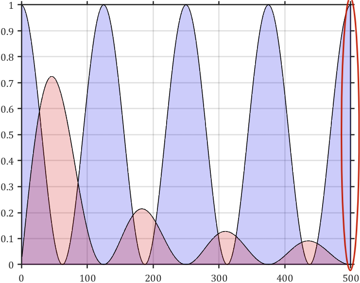
¿Hay alguna forma de no mostrar esta escala? ? Aunque podemos obtener BoxFrame, este no tiene una propiedad de escala, por lo que pensamos en dibujar una línea recta directamente, al mismo tiempo, para mantener la posición de la línea donde debería estar el marco al arrastrar la imagen, agregamos un monitor al área de coordenadas actual, más o menos así:
function testBox
t  = linspace(pi/100,4*pi,500);
y1 = cos(t).^2;
y2 = sin(t).^2./t;
% 基础绘图
hold on
area(y1,'LineWidth',.8,'FaceColor',[0,0,.9],'FaceAlpha',.2)
area(y2,'LineWidth',.8,'FaceColor',[.8,0,0],'FaceAlpha',.2)
% 坐标区域基础修饰
ax=gca; grid on; box on
ax.FontName  = 'Cambria';
ax.TickDir   = 'out';
ax.LineWidth = 1;
% 绘制可跟随移动的框线
ax=gca; box off
XLineHdl=plot(ax,ax.XLim([1,2]),ax.YLim([2,2]),'LineWidth',1,'Color',[0,0,0]);
YLineHdl=plot(ax,ax.XLim([2,2]),ax.YLim([1,2]),'LineWidth',1,'Color',[0,0,0]);
addlistener(ax,'MarkedClean',@changeLinePos)
function changeLinePos(~,~)
    set(XLineHdl,'XData',ax.XLim([1,2]),'YData',ax.YLim([2,2]))
    set(YLineHdl,'XData',ax.XLim([2,2]),'YData',ax.YLim([1,2]))
end
end

Eso sí, no nos conviene mucho usarlo así, podemos encapsularlo como una función:
function addBox
ax=gca; box off
XLineHdl=plot(ax,ax.XLim([1,2]),ax.YLim([2,2]),'LineWidth',ax.LineWidth,'Color',ax.XColor);
YLineHdl=plot(ax,ax.XLim([2,2]),ax.YLim([1,2]),'LineWidth',ax.LineWidth,'Color',ax.YColor);
addlistener(ax,'MarkedClean',@changeLinePos)
function changeLinePos(~,~)
    set(XLineHdl,'XData',ax.XLim([1,2]),'YData',ax.YLim([2,2]))
    set(YLineHdl,'XData',ax.XLim([2,2]),'YData',ax.YLim([1,2]))
end
end
De esta manera, después de dibujar la imagen, agregue una línea de addBox() al final. El color y el grosor del cuadro coincidirán con el color del eje:
t  = linspace(pi/100,4*pi,500);
y1 = cos(t).^2;
y2 = sin(t).^2./t;
% 基础绘图
hold on
area(y1,'LineWidth',.8,'FaceColor',[0,0,.9],'FaceAlpha',.2)
area(y2,'LineWidth',.8,'FaceColor',[.8,0,0],'FaceAlpha',.2)
% 坐标区域基础修饰
ax=gca; grid on; box on
ax.FontName  = 'Cambria';
ax.TickDir   = 'out';
ax.LineWidth = 1;
ax.XColor    = [0,0,.8];
ax.YColor    = [.8,0,0];

addBox()

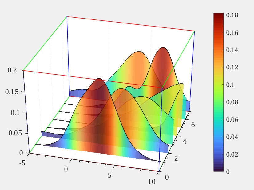
4 El color de la caja 3D.
Supongamos que escribimos el siguiente código:
% 获取数据
X1=normrnd(2,2,1,50);
X2=[normrnd(4,4,1,50),normrnd(5,2,1,50)];
X3=[normrnd(6,2,1,50),normrnd(8,4,1,50)];
X4=[normrnd(12,1,1,50),normrnd(12,4,1,50)];
X5=[normrnd(10,2,1,50),normrnd(10,4,1,50)];
X6=[normrnd(7,2,1,50),normrnd(7,4,1,50)];
X7=[normrnd(4,2,1,50),normrnd(4,4,1,50)];
Data={

    X1,X2,X3,X4,X5,X6,X7};
Y=zeros(7,500);
for i=1:length(Data)
    tX=Data{

    i};tX=tX(:)';
    [F,Xi]=ksdensity(tX,linspace(-5,10,500));
    Y(i,:)=F;
end
X=Xi;

YLim=[min(min(Y)),max(max(Y))];
% 构造并绘制网格
[XMesh,YMesh]=meshgrid(X,linspace(YLim(1),YLim(2),1000));
hold on
for i=1:size(Y,1)
    YMeshA=repmat(Y(i,:),[1000,1]);
    CMesh=nan.*XMesh;
    YMeshD=YMeshA-YLim(1);
    CMesh(YMesh>=YLim(1)&YMesh<=YMeshA)=YMeshD(YMesh>=YLim(1)&YMesh<=YMeshA);
    surf(XMesh,XMesh.*0+i,YMesh,'EdgeColor','none','CData',CMesh,'FaceColor','flat','FaceAlpha',.8)
end

% 绘制折线图
for i=1:size(Y,1)
    plot3(X,X.*0+i,Y(i,:),'LineWidth',1,'Color',[0,0,0,.8])
end

% 设置配色
colorList=turbo(64);
% colorList=slanCM(110,64);
colormap(colorList)
colorbar

% 坐标区域修饰
ax=gca;hold on;box on
ax.XGrid='on';
ax.YGrid='on';
ax.XMinorTick='on';
ax.YMinorTick='on';
ax.LineWidth=.8;
ax.GridLineStyle='-.';
ax.FontName='Cambria';
ax.FontSize=12;
ax.GridAlpha=.03;
ax.Projection='perspective';
ax.GridAlpha=.05;
ax.BoxStyle='full';
view(16,36)

El color de cada línea de marco se puede establecer a través de la propiedad boxFrame:
% 设置框线颜色
ax=gca;
pause(1e-6);
ax.BoxFrame.XColor=[1,0,0];
ax.BoxFrame.YColor=[0,1,0];
ax.BoxFrame.ZColor=[0,0,1];
Se puede ver que solo la línea del marco cambia de color, pero la línea del eje no cambia de color. Esta propiedad es solo una propiedad de visualización y el color no se puede conservar al guardar, por lo que se recomienda dibujar una línea dura:
Toma una pequeña parte de lo que escribí antes y vuelve a mencionarlo:
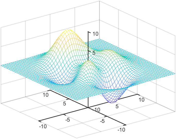
5 Cambiar la posición del eje de trazado 3D
parahAxes=gca
- hAxes.XRuler.FirstCrossoverValue
La posición del eje X en el eje Y - hAxes.XRuler.SecondCrossoverValue
La posición del eje X en el eje Z - hAxes.YRuler.FirstCrossoverValue
La posición del eje Y en el eje X - hAxes.YRuler.SecondCrossoverValue
La posición del eje Y en el eje Z - hAxes.ZRuler.FirstCrossoverValue
La posición del eje Z en el eje X - hAxes.ZRuler.SecondCrossoverValue
La posición del eje Z en el eje Y
Un ejemplo:
N = 49;
X = linspace(-10,10,N);
Z = peaks(N);
mesh(X,X,Z);

hAxes=gca;
hAxes.LineWidth=1.5;
hAxes.XRuler.FirstCrossoverValue  = 0; % X轴在Y轴上的位置
hAxes.YRuler.FirstCrossoverValue  = 0; % Y轴在X轴上的位置
hAxes.ZRuler.FirstCrossoverValue  = 0; % Z轴在X轴上的位置
hAxes.ZRuler.SecondCrossoverValue = 0; % Z轴在Y轴上的位置
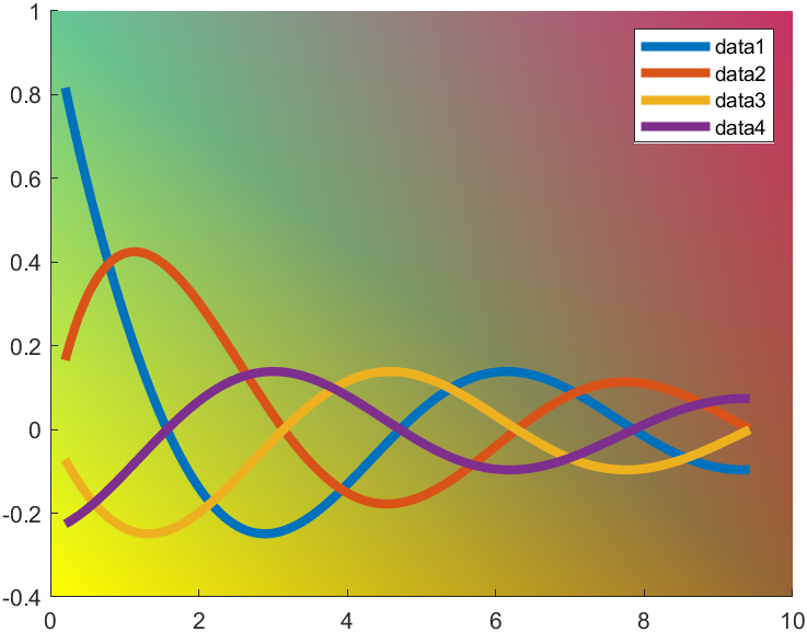
6 Modificar el fondo del área de coordenadas
Sabemos que al establecer
set(gca,'Color',[1,0,0])
El color de fondo se establece de forma similar, pero es solo un color sólido, entonces, ¿hay alguna forma de cambiar el color de fondo a un color degradado?
t=0.2:0.01:3*pi;

hold on
plot(t,cos(t)./(1+t),'LineWidth',4)
plot(t,sin(t)./(1+t),'LineWidth',4)
plot(t,cos(t+pi/2)./(1+t+pi/2),'LineWidth',4)
plot(t,cos(t+pi)./(1+t+pi),'LineWidth',4)
legend


ax=gca;pause(1e-16);% Backdrop建立需要一定时间因此pause一下很重要
% 四列分别为四个角的颜色
% 使用4xN大小颜色矩阵
% 四行分别是R,G,B,和透明度
colorData = uint8([255, 150, 200, 100; ...
                   255, 100,  50, 200; ...
                     0,  50, 100, 150; ...
                   102, 150, 200,  50]);
set(ax.Backdrop.Face, 'ColorBinding','interpolated','ColorData',colorData);
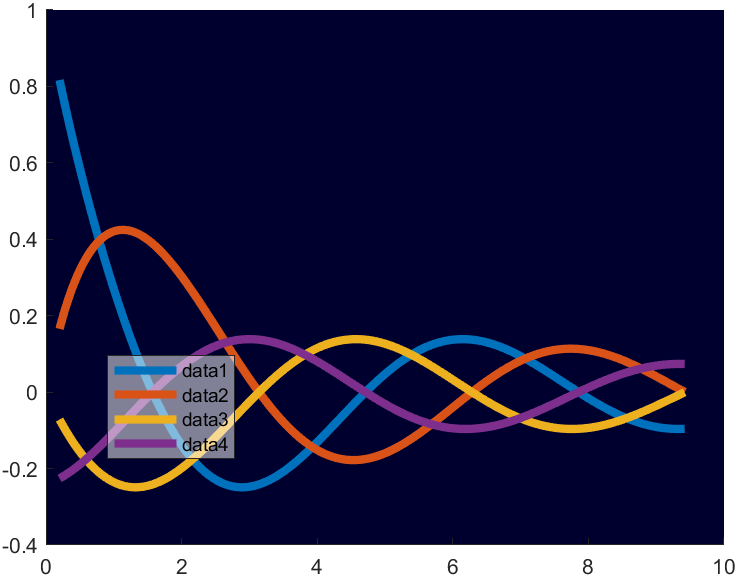
7 Leyenda de translucidez y degradado
t=0.2:0.01:3*pi;

hold on
plot(t,cos(t)./(1+t),'LineWidth',4)
plot(t,sin(t)./(1+t),'LineWidth',4)
plot(t,cos(t+pi/2)./(1+t+pi/2),'LineWidth',4)
plot(t,cos(t+pi)./(1+t+pi),'LineWidth',4)
hLegend=legend();
% 设置图例为半透明
pause(1e-16)
set(hLegend.BoxFace,'ColorType','truecoloralpha','ColorData',uint8(255*[1;1;1;.5]));

set(gca,'Color',[0,0,.18]);
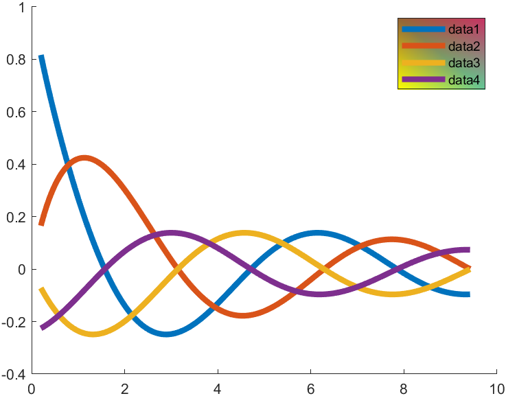
Por supuesto, también puede ser elegante:
t=0.2:0.01:3*pi;
hold on
plot(t,cos(t)./(1+t),'LineWidth',4)
plot(t,sin(t)./(1+t),'LineWidth',4)
plot(t,cos(t+pi/2)./(1+t+pi/2),'LineWidth',4)
plot(t,cos(t+pi)./(1+t+pi),'LineWidth',4)
hLegend=legend();

% 设置图例为渐变色
pause(1e-16)
colorData = uint8([255, 150, 200, 100; ...
                   255, 100,  50, 200; ...
                     0,  50, 100, 150; ...
                   102, 150, 200,  50]);
set(hLegend.BoxFace,'ColorBinding','interpolated','ColorData',colorData)
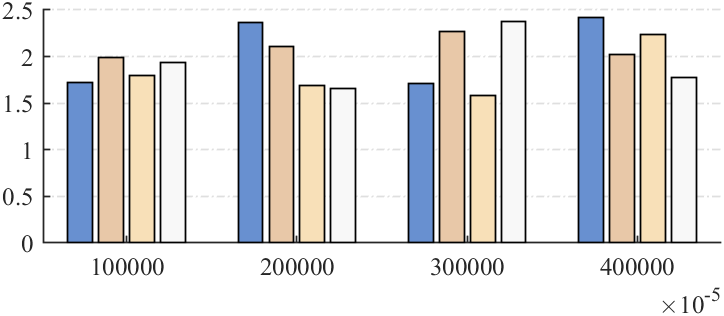
8 notación científica para etiquetas de eje
Que pasa si queremos expresar el valor de la escala en notación científica, si escribimos el siguiente código:
rng(5)
% 随机生成数据
X=1.5+rand(4,4);
% 基础绘图
ax=gca;hold on;
bHdl=bar(X,'LineWidth',.8);
% 修改配色
CList=[0.4078    0.5647    0.8157
    0.9098    0.7843    0.6588
    0.9725    0.8784    0.7216
    0.9725    0.9725    0.9725];
bHdl(1).FaceColor=CList(1,:);
bHdl(2).FaceColor=CList(2,:);
bHdl(3).FaceColor=CList(3,:);
bHdl(4).FaceColor=CList(4,:);
% 坐标区域修饰
ax.FontName='Times New Roman';
ax.LineWidth=.8;
ax.FontSize=12;
ax.YGrid='on';
ax.GridLineStyle='-.';
ax.XTick=1:4;
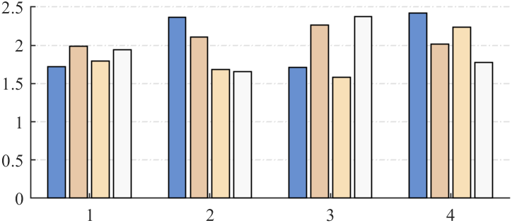
Escriba el siguiente código al final para usar notación científica:
ax=gca;
ax.XRuler.Exponent=-5;

ax=gca;
ax.XRuler.Exponent=5;
9 fórmulas de etiquetas más complejas
La etiqueta de escala también se puede cambiar para admitir látex, o la función de dibujo anterior, y agregar al final:
ax.XRuler.TickLabelInterpreter='latex';
ax.XTickLabel={

    '$\Delta A B C$','$\frac{n!}{r!(n-r)!} $','$\left(\begin{array}{cc}A& B\\C& D\end{array}\right)$','$E = n{

    { \Delta \Phi } \over {\Delta {t} }}  $'}

10 Mostrar subpestañas
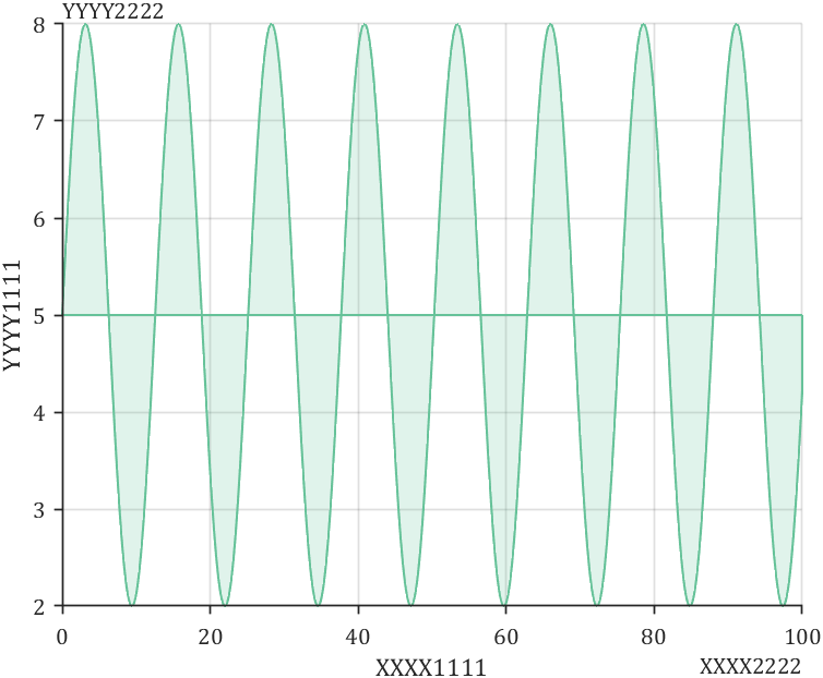
Finalmente, hablemos sobre cómo mostrar las etiquetas secundarias del eje X y del eje Y:
x = linspace(0,100,1000);
y = 5 + 3*sin(x./2);
fill([x x(end)],[y y(1)],[0.40 0.76 0.60],'FaceAlpha',.2,...
    'LineWidth',1,'EdgeColor',[0.40 0.76 0.60])
% 坐标区域基础修饰
ax=gca; grid on;
ax.FontName  = 'Cambria';
ax.TickDir   = 'out';
ax.LineWidth = .8;
ax.Box       = 'off';

% 显示次标签
ax=gca;
% X轴主次标签
xlabel('XXXX1111')
ax.XRuler.SecondaryLabel.String='XXXX2222';
ax.XRuler.SecondaryLabel.Visible='on';
% Y轴主次标签
ylabel('YYYY1111')
ax.YRuler.SecondaryLabel.String='YYYY2222';
ax.YRuler.SecondaryLabel.Visible='on';
encima
¡Este número es lo suficientemente largo y el próximo número puede agregar otras operaciones escandalosas en MATLAB! ! !