Introducción al aprendizaje profundo: teoría e implementación basadas en Python Capítulo 4 Aprendizaje en redes neuronales

import numpy as np
import matplotlib.pylab as plt

# 均方误差的实现
def mean_squared_error(y, t):
    return 0.5 * np.num((y - t) ** 2)

# 交叉熵误差
def cross_entropy_error(y, t):
    delta = 1e-7
    return -np.sum(t*np.log(y+delta))

# mini-batch版交叉熵误差的实现
def cross_entropy_error(y, t):
    if y.ndim == 1:
        t = t.reshape(1, t.size)
        y = y.reshape(1, y.size)
        
    batch_size = y.shape[0]
    return -np.sum(t*np.log(y+1e-7)) / batch_size

# 中心差分
def numerical_diff(f, x):
    h = 1e-4 #0.0001
    return (f(x+h) - f(x-h)) / (2*h)

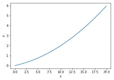
#数值微分的例子
def function_1(x):
    return 0.01*x**2 + 0.1*x

x = np.arange(0.0, 20.0, 0.1) # 以0.1为单位，从0到20的数组x
y = function_1(x)
plt.xlabel("x")
plt.ylabel("y")
plt.plot(x, y)
plt.show()

print(numerical_diff(function_1, 5))
print(numerical_diff(function_1, 10))

0.1999999999990898
0.2999999999986347

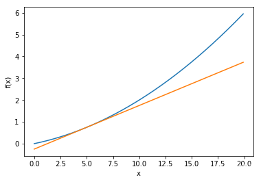
# 画在函数某一点的切线
def tangent_line(f, x):
    d = numerical_diff(f, x)
    print(d)
    y = f(x) - d*x # 在这里y是截距，d是斜率
    return lambda t: d*t + y

x = np.arange(0.0, 20.0, 0.1) # 以0.1为单位，从0到20的数组x
y = function_1(x)
plt.xlabel("x")
plt.ylabel("f(x)")

tf = tangent_line(function_1, 5)
y2 = tf(x)

plt.plot(x, y)
plt.plot(x, y2)
plt.show()

0.1999999999990898

np.array([3.0, 4.0])

array([3., 4.])

# 偏导数示例函数: 两个数的平方和
def function_2(x):
    # 下一条更好
    # return np.sum(x**2)
    return x[0]**2 + x[1]**2

def numerical_gradient(f, x):
    h = 1e-4 # 0.0001
    grad = np.zeros_like(x) # 生成和x形状相同的数组
    
    for idx in range(x.size):
        tmp_val = x[idx]
        # f(x+h)的计算
        x[idx] = tmp_val + h
        fxh1 = f(x)
        
        # f(x-h)的计算
        x[idx] = tmp_val - h
        fxh2 = f(x)
        
        grad[idx] = (fxh1 - fxh2) / (2*h)
        x[idx] = tmp_val
        
    return grad

numerical_gradient(function_2, np.array([3.0, 4.0]))

array([6., 8.])

# 梯度下降法
def gradient_descent(f, init_x, lr=0.01, step_num=100):
    x = init_x
    for i in range(step_num):
        grad = numerical_gradient(f,x)
        x -= lr * grad
        
    return x

Use el método de gradiente para encontrar $$f(x_0+X_1)={X_0}^2+{X_1}^2$$

def function_2(x):
    return x[0]**2 + x[1]**2

init_x = np.array([-3.0, 4.0])
gradient_descent(function_2, init_x=init_x, lr=0.1, step_num=100)

array([-6.11110793e-10,  8.14814391e-10])

# 神经网络的梯度
import sys,os
import numpy as np
from common.functions import softmax, cross_entropy_error
from common.gradient import numerical_gradient

class simpleNet:
    def __init__(self):
        self.W = np.random.randn(2,3) # 用高斯分布进行初始化
        
    def predict(self, x):
        return np.dot(x, self.W)
    
    def loss(self, x, t):
        z = self.predict(x)
        y = softmax(z)
        loss = cross_entropy_error(y, t)
        
        return loss

net = simpleNet()
print(net.W)
x = np.array([0.6, 0.9])
p = net.predict(x)
print(p)
print(np.argmax(p))
t = np.array([0, 0, 1])
net.loss(x,t)

[[-1.77081556  1.3171629  -0.88412637]
 [ 1.73434721 -0.27546099  1.6995778 ]]
[0.49842315 0.54238284 0.9991442 ]
2





0.8062188854106839

def f(W):
    return net.loss(x,t)

# f = lambda w: net.loss(x, t)

dW = numerical_gradient(f, net.W)
print(dW)

[[ 0.16238812  0.16968588 -0.332074  ]
 [ 0.24358218  0.25452882 -0.498111  ]]

# 两层神经网络的类
import sys, os
from common.functions import *
from common.gradient import numerical_gradient

class TwoLayerNet:
    def __init__(self, input_size, hidden_size, output_size,
                 weight_init_std=0.01):
        # 初始化权重
        self.params = {
    
    }
        self.params['W1'] = weight_init_std * \
                            np.random.randn(input_size, hidden_size)
        self.params['b1'] = np.zeros(hidden_size)
        self.params['W2'] = weight_init_std * \
                            np.random.randn(hidden_size, output_size)
        self.params['b2'] = np.zeros(output_size)
        
    def predict(self, x):
        W1, W2 = self.params['W1'], self.params['W2']
        b1, b2 = self.params['b1'], self.params['b2']
        
        a1 = np.dot(x, W1) + b1
        z1 = sigmoid(a1)
        a2 = np.dot(z1, W2) + b2
        y = softmax(a2)
        
        return y
    
    # x:输入数据， t：监督数据
    def loss(self, x, t):
        y = self.predict(x)
        
        return cross_entropy_error(y, t)
    
    def accuracy(self, x, t):
        y = self.predict(x)
        y = np.argmax(y, axis=1)
        t = np.argmax(t, axis=1)
        
        accuracy = np.sum(y == t) / float(x.shape[0])
        return accuracy
    
    def numerical_gradient(self, x, t):
        loss_W = lambda W: self.loss(x, t)
        
        grads = {
    
    }
        grads['W1'] = numerical_gradient(loss_W, self.params['W1'])
        grads['b1'] = numerical_gradient(loss_W, self.params['b1'])
        grads['W2'] = numerical_gradient(loss_W, self.params['W2'])
        grads['b2'] = numerical_gradient(loss_W, self.params['b2'])
        
        return grads
    
    def gradient(self, x, t):
        W1, W2 = self.params['W1'], self.params['W2']
        b1, b2 = self.params['b1'], self.params['b2']
        grads = {
    
    }
        
        batch_num = x.shape[0]
        
        #forward
        a1 = np.dot(x, W1) + b1
        z1 = sigmoid(a1)
        a2 = np.dot(z1, W2) + b2
        y = softmax(a2)
        
        #backward
        dy = (y-t)/batch_num
        grads['W2'] = np.dot(z1.T, dy)
        grads['b2'] = np.sum(dy, axis=0)
        
        da1 = np.dot(dy, W2.T)
        dz1 = sigmoid_grad(a1) * da1
        grads['W1'] = np.dot(x.T, dz1)
        grads['b1'] = np.sum(dz1, axis = 0)
        
        return grads

# mini-batch的实现
import numpy as np
from mnist import load_mnist

(x_train, t_train), (x_test, t_test) = load_mnist(normalize=True, one_hot_label = True)

train_loss_list = []
train_acc_list = []
test_acc_list = []
iter_per_epoch = max(train_size / batch_size, 1)

iters_num = 10000
train_size = x_train.shape[0]
batch_size = 100
learning_rate = 0.1
network = TwoLayerNet(input_size=784, hidden_size=50, output_size=10)

for i in range(iters_num):
    # 获取mini-batch
    batch_mask = np.random.choice(train_size, batch_size)
    x_batch = x_train[batch_mask]
    t_batch = t_train[batch_mask]
    
    # 计算梯度
    #grad = network.numerical_gradient(x_batch, t_batch)
    grad = network.gradient(x_batch, t_batch)

    for key in ('W1', 'b1', 'W2', 'b2'):
        network.params[key] -= learning_rate * grad[key]
        
    # 记录学习过程
    loss = network.loss(x_batch, t_batch)
    train_loss_list.append(loss)

    # 计算每个epoch的识别精度
    if i % iter_per_epoch == 0:
        train_acc = network.accuracy(x_train, t_train)
        test_acc = network.accuracy(x_test, t_test)
        train_acc_list.append(train_acc)
        test_acc_list.append(test_acc)
        print("train acc, test acc | " + str(train_acc) + ", " + str(test_acc))

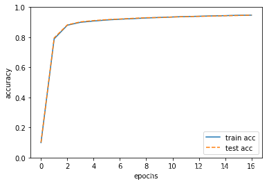
train acc, test acc | 0.09915, 0.1009
train acc, test acc | 0.7893833333333333, 0.7955
train acc, test acc | 0.8799333333333333, 0.8822
train acc, test acc | 0.8994666666666666, 0.9022
train acc, test acc | 0.9077833333333334, 0.9106
train acc, test acc | 0.9147666666666666, 0.917
train acc, test acc | 0.9200666666666667, 0.9212
train acc, test acc | 0.9235333333333333, 0.9257
train acc, test acc | 0.9283166666666667, 0.93
train acc, test acc | 0.9314833333333333, 0.9308
train acc, test acc | 0.93475, 0.9346
train acc, test acc | 0.9373333333333334, 0.9371
train acc, test acc | 0.9395666666666667, 0.939
train acc, test acc | 0.9419166666666666, 0.9406
train acc, test acc | 0.9436666666666667, 0.943
train acc, test acc | 0.9460166666666666, 0.9445
train acc, test acc | 0.9468833333333333, 0.9473

markers = {
    
    'train': 'o', 'test':'s'}
x = np.arange(len(train_acc_list))
plt.plot(x, train_acc_list, label='train acc')
plt.plot(x, test_acc_list, label='test acc', linestyle='--')
plt.xlabel("epochs")
plt.ylabel("accuracy")
plt.ylim(0, 1.0)
plt.legend(loc='lower right')
plt.show()