Reconocimiento facial
Reconocimiento facial para la casa feliz
from keras.models import Sequential
from keras.layers import Conv2D, ZeroPadding2D, Activation, Input, concatenate
from keras.models import Model
from keras.layers.normalization import BatchNormalization
from keras.layers.pooling import MaxPooling2D, AveragePooling2D
from keras.layers.merge import Concatenate
from keras.layers.core import Lambda, Flatten, Dense
from keras.initializers import glorot_uniform
from keras.engine.topology import Layer
from keras import backend as K
K.set_image_data_format('channels_first')
import cv2
import os
import numpy as np
from numpy import genfromtxt
import pandas as pd
import tensorflow as tf
from fr_utils import *
from inception_blocks_v2 import *

%matplotlib inline
%load_ext autoreload
%autoreload 2

np.set_printoptions(threshold=np.nan)
0 - Verificación de la cara ingenua
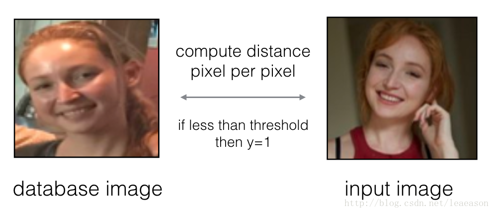
En la Verificación facial, se te dan dos imágenes y tienes que saber si son de la misma persona. La forma más sencilla de hacer esto es comparar las dos imágenes píxel por píxel. Si la distancia entre las imágenes en bruto es inferior al umbral elegido, ¡puede ser la misma persona!
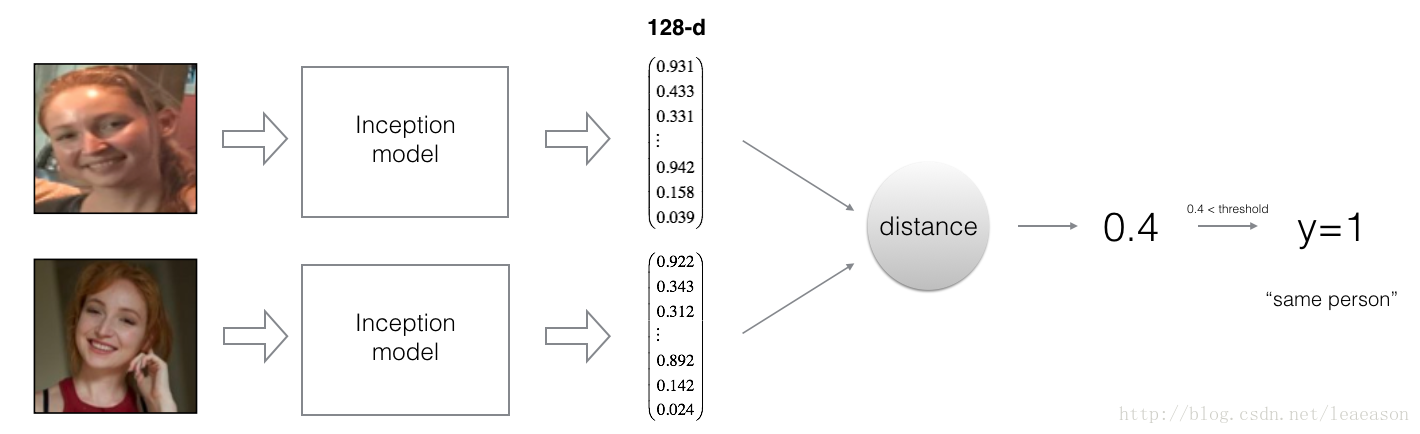
1 - Codificación de imágenes faciales en un vector de 128 dimensiones
1.1 - Usando un ConvNet para calcular codificaciones
El modelo FaceNet requiere muchos datos y mucho tiempo para entrenar. Entonces, siguiendo la práctica común en entornos de aprendizaje profundo aplicados, simplemente carguemos pesos que otra persona ya haya entrenado. La arquitectura de red sigue el modelo de inicio de Szegedy et al. Hemos proporcionado una implementación de red de inicio. Puede buscar en el archivo inception_blocks.py para ver cómo se implementa (hágalo yendo a "Archivo-> Abrir ..." en la parte superior del cuaderno Jupyter).
FRmodel = faceRecoModel(input_shape=(3, 96, 96))
print("Total Params:", FRmodel.count_params())
Parámetros totales: 3743280
Al usar una capa de 128 neuronas totalmente conectadas como su última capa, el modelo asegura que la salida es un vector de codificación de tamaño 128. Luego usa las codificaciones para comparar las dos imágenes de la siguiente manera:
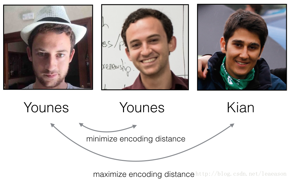
Entonces, una codificación es una buena si:
Las codificaciones de dos imágenes de la misma persona son bastante similares entre sí.
Las codificaciones de dos imágenes de diferentes personas son muy diferentes.
La función de pérdida de triplete formaliza esto e intenta "empujar" las codificaciones de dos imágenes de la misma persona (Ancla y Positiva) más cerca, mientras "tira" de las codificaciones de dos imágenes de diferentes personas (Ancla, Negativa) más separadas.
1.2 - La pérdida de triplete
# GRADED FUNCTION: triplet_loss

def triplet_loss(y_true, y_pred, alpha = 0.2):
    """
    Implementation of the triplet loss as defined by formula (3)

    Arguments:
    y_true -- true labels, required when you define a loss in Keras, you don't need it in this function.
    y_pred -- python list containing three objects:
            anchor -- the encodings for the anchor images, of shape (None, 128)
            positive -- the encodings for the positive images, of shape (None, 128)
            negative -- the encodings for the negative images, of shape (None, 128)

    Returns:
    loss -- real number, value of the loss
    """

    anchor, positive, negative = y_pred[0], y_pred[1], y_pred[2]

    ### START CODE HERE ### (≈ 4 lines)
    # Step 1: Compute the (encoding) distance between the anchor and the positive
    pos_dist = tf.reduce_sum(tf.square(tf.subtract(y_pred[0],y_pred[1])))
    # Step 2: Compute the (encoding) distance between the anchor and the negative
    neg_dist = tf.reduce_sum(tf.square(tf.subtract(y_pred[0],y_pred[2])))
    # Step 3: subtract the two previous distances and add alpha.
    basic_loss = tf.add(tf.subtract(pos_dist,neg_dist),alpha)
    # Step 4: Take the maximum of basic_loss and 0.0. Sum over the training examples.
    loss = tf.reduce_sum(tf.maximum(basic_loss,0.0))
    ### END CODE HERE ###

    return loss
with tf.Session() as test:
tf.set_random_seed(1)
y_true = (None, None, None)
y_pred = (tf.random_normal([3, 128], mean=6, stddev=0.1, seed = 1),
tf.random_normal([3, 128], mean=1, stddev=1, seed = 1),
tf.random_normal([3, 128], mean=3, stddev=4, seed = 1))
loss = triplet_loss(y_true, y_pred)
print("loss = " + str(loss.eval()))pérdida = 350.026
2 - Cargando el modelo entrenado
FRmodel.compile(optimizer = 'adam', loss = triplet_loss, metrics = ['accuracy'])
load_weights_from_FaceNet(FRmodel)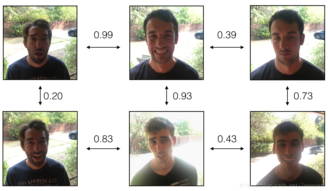
3 - Aplicando el modelo
De vuelta a la casa feliz! Los residentes viven felizmente desde que implementaste el reconocimiento de felicidad para la casa en una asignación anterior.
Sin embargo, surgen varios problemas: The Happy House se puso tan feliz que todas las personas felices del vecindario vendrán a pasar el rato en tu sala de estar. Se está llenando de gente, lo que está teniendo un impacto negativo en los residentes de la casa. Todas estas personas felices al azar también están comiendo toda tu comida.
Por lo tanto, decide cambiar la política de entrada a la puerta, y no solo dejar que ingresen personas felices al azar, ¡incluso si son felices! En cambio, le gustaría construir un sistema de verificación de Rostros para permitir que solo entren personas de una lista específica. Para ser admitido, cada persona debe deslizar una tarjeta de identificación (tarjeta de identificación) para identificarse en la puerta. El sistema de reconocimiento facial luego verifica que son quienes dicen ser.
3.1 - Verificación facial
database = {}
database["danielle"] = img_to_encoding("images/danielle.png", FRmodel)
database["younes"] = img_to_encoding("images/younes.jpg", FRmodel)
database["tian"] = img_to_encoding("images/tian.jpg", FRmodel)
database["andrew"] = img_to_encoding("images/andrew.jpg", FRmodel)
database["kian"] = img_to_encoding("images/kian.jpg", FRmodel)
database["dan"] = img_to_encoding("images/dan.jpg", FRmodel)
database["sebastiano"] = img_to_encoding("images/sebastiano.jpg", FRmodel)
database["bertrand"] = img_to_encoding("images/bertrand.jpg", FRmodel)
database["kevin"] = img_to_encoding("images/kevin.jpg", FRmodel)
database["felix"] = img_to_encoding("images/felix.jpg", FRmodel)
database["benoit"] = img_to_encoding("images/benoit.jpg", FRmodel)
database["arnaud"] = img_to_encoding("images/arnaud.jpg", FRmodel)
# GRADED FUNCTION: verify
def verify(image_path, identity, database, model):
"""
Function that verifies if the person on the "image_path" image is "identity".
Arguments:
image_path -- path to an image
identity -- string, name of the person you'd like to verify the identity. Has to be a resident of the Happy house.
database -- python dictionary mapping names of allowed people's names (strings) to their encodings (vectors).
model -- your Inception model instance in Keras
Returns:
dist -- distance between the image_path and the image of "identity" in the database.
door_open -- True, if the door should open. False otherwise.
"""
### START CODE HERE ###
# Step 1: Compute the encoding for the image. Use img_to_encoding() see example above. (≈ 1 line)
encoding = img_to_encoding(image_path,model)
# Step 2: Compute distance with identity's image (≈ 1 line)
dist = np.linalg.norm(encoding-database[identity])
# Step 3: Open the door if dist < 0.7, else don't open (≈ 3 lines)
if dist<0.7:
print("It's " + str(identity) + ", welcome home!")
door_open = True
else:
print("It's not " + str(identity) + ", please go away")
door_open = False
### END CODE HERE ###
return dist, door_openverify("images/camera_0.jpg", "younes", database, FRmodel)
3.2 - Reconocimiento facial
Su sistema de verificación de rostro funciona principalmente bien. Pero desde que le robaron su tarjeta de identificación, ¡cuando regresó a la casa esa noche no pudo entrar!
Para reducir tales travesuras, le gustaría cambiar su sistema de verificación facial a un sistema de reconocimiento facial. De esta manera, ya nadie tiene que llevar una tarjeta de identificación. ¡Una persona autorizada puede simplemente caminar hasta la casa, y la puerta principal se abrirá para ellos!
Implementará un sistema de reconocimiento facial que toma como entrada una imagen y determina si es una de las personas autorizadas (y si es así, quién). A diferencia del sistema de verificación facial anterior, ya no obtendremos el nombre de una persona como otra entrada.
Ejercicio: Implemente who_is_it (). Deberá seguir los siguientes pasos:
Calcule la codificación de destino de la imagen desde image_path
Encuentre la codificación de la base de datos que tiene la distancia más pequeña con la codificación de destino.
Inicialice la variable min_dist a un número suficientemente grande (100). Le ayudará a realizar un seguimiento de cuál es la codificación más cercana a la codificación de la entrada.
Recorra los nombres y codificaciones del diccionario de la base de datos. Para usar el bucle for (name, db_enc) en database.items ().
Calcule la distancia L2 entre la "codificación" de destino y la "codificación" actual de la base de datos.
Si esta distancia es menor que min_dist, establezca min_dist en dist, y la identidad como nombre.
# GRADED FUNCTION: who_is_it

def who_is_it(image_path, database, model):
    """
    Implements face recognition for the happy house by finding who is the person on the image_path image.

    Arguments:
    image_path -- path to an image
    database -- database containing image encodings along with the name of the person on the image
    model -- your Inception model instance in Keras

    Returns:
    min_dist -- the minimum distance between image_path encoding and the encodings from the database
    identity -- string, the name prediction for the person on image_path
    """

    ### START CODE HERE ###

    ## Step 1: Compute the target "encoding" for the image. Use img_to_encoding() see example above. ## (≈ 1 line)
    encoding = img_to_encoding(image_path,model)

    ## Step 2: Find the closest encoding ##

    # Initialize "min_dist" to a large value, say 100 (≈1 line)
    min_dist = 100

    # Loop over the database dictionary's names and encodings.
    for (name, db_enc) in database.items():

        # Compute L2 distance between the target "encoding" and the current "emb" from the database. (≈ 1 line)
        dist = np.linalg.norm(encoding-db_enc)

        # If this distance is less than the min_dist, then set min_dist to dist, and identity to name. (≈ 3 lines)
        if dist<min_dist:
            min_dist = dist
            identity = name

    ### END CODE HERE ###

    if min_dist > 0.7:
        print("Not in the database.")
    else:
        print ("it's " + str(identity) + ", the distance is " + str(min_dist))

return min_dist, identitywho_is_it("images/camera_0.jpg", database, FRmodel)Aprendizaje profundo y arte: transferencia de estilo neuronal
Bienvenido a la segunda tarea de esta semana. En esta tarea, aprenderá sobre la transferencia de estilo neuronal. Este algoritmo fue creado por Gatys et al. (2015) ( https://arxiv.org/abs/1508.06576 ).
En esta tarea, usted:
Implementará el algoritmo de transferencia de estilo neural
Generará imágenes artísticas novedosas utilizando su algoritmo
La mayoría de los algoritmos que ha estudiado optimizan una función de costo para obtener un conjunto de valores de parámetros. ¡En Neural Style Transfer, optimizará una función de costo para obtener valores de píxeles!
import os
import sys
import scipy.io
import scipy.misc
import matplotlib.pyplot as plt
from matplotlib.pyplot import imshow
from PIL import Image
from nst_utils import *
import numpy as np
import tensorflow as tf

%matplotlib inline
1 - Declaración del problema
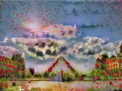
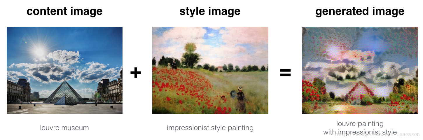
Neural Style Transfer (NST) es una de las técnicas más divertidas en el aprendizaje profundo. Como se ve a continuación, combina dos imágenes, a saber, una imagen de "contenido" (C) y una imagen de "estilo" (S), para crear una imagen "generada" (G). La imagen generada G combina el "contenido" de la imagen C con el "estilo" de la imagen S.
En este ejemplo, va a generar una imagen del museo del Louvre en París (imagen de contenido C), mezclada con una pintura de Claude Monet, líder del movimiento impresionista (imagen de estilo S).
2 - Aprendizaje de transferencia
Neural Style Transfer (NST) utiliza una red convolucional previamente capacitada, y se suma a eso. La idea de usar una red capacitada en una tarea diferente y aplicarla a una nueva tarea se llama aprendizaje de transferencia.
Siguiendo el documento original de NST ( https://arxiv.org/abs/1508.06576 ), utilizaremos la red VGG. Específicamente, utilizaremos VGG-19, una versión de 19 capas de la red VGG. Este modelo ya ha sido entrenado en la gran base de datos ImageNet y, por lo tanto, ha aprendido a reconocer una variedad de características de bajo nivel (en las capas anteriores) y características de alto nivel (en las capas más profundas).
Ejecute el siguiente código para cargar parámetros desde el modelo VGG. Esto puede tardar unos pocos segundos.
3 - Transferencia de estilo neural
3.1 - Calcular el costo del contenido
content_image = scipy.misc.imread("images/louvre.jpg")
imshow(content_image)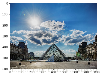
# GRADED FUNCTION: compute_content_cost

def compute_content_cost(a_C, a_G):
    """
    Computes the content cost

    Arguments:
    a_C -- tensor of dimension (1, n_H, n_W, n_C), hidden layer activations representing content of the image C
    a_G -- tensor of dimension (1, n_H, n_W, n_C), hidden layer activations representing content of the image G

    Returns:
    J_content -- scalar that you compute using equation 1 above.
    """

    ### START CODE HERE ###
    # Retrieve dimensions from a_G (≈1 line)
    m, n_H, n_W, n_C = a_G.get_shape().as_list()

    # Reshape a_C and a_G (≈2 lines)
    a_C_unrolled = tf.reshape(a_C,shape=(n_H* n_W,n_C))
    a_G_unrolled = tf.reshape(a_G,shape=(n_H* n_W,n_C))

    # compute the cost with tensorflow (≈1 line)
    J_content = tf.reduce_sum(tf.square(tf.subtract(a_C_unrolled,a_G_unrolled)))/(4*n_H*n_W*n_C)
    ### END CODE HERE ###

return J_contenttf.reset_default_graph()
with tf.Session() as test:
tf.set_random_seed(1)
a_C = tf.random_normal([1, 4, 4, 3], mean=1, stddev=4)
a_G = tf.random_normal([1, 4, 4, 3], mean=1, stddev=4)
J_content = compute_content_cost(a_C, a_G)
print("J_content = " + str(J_content.eval()))J_content = 6.76559
3.2 - Calcular el costo del estilo
3.2.1 - Matriz de estilo
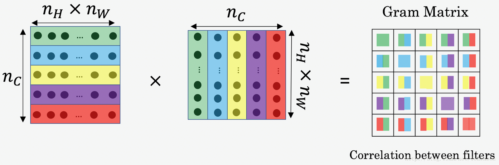
# GRADED FUNCTION: gram_matrix

def gram_matrix(A):
    """
    Argument:
    A -- matrix of shape (n_C, n_H*n_W)

    Returns:
    GA -- Gram matrix of A, of shape (n_C, n_C)
    """

    ### START CODE HERE ### (≈1 line)
    GA = tf.matmul(A,tf.transpose(A))
    ### END CODE HERE ###

return GAtf.reset_default_graph()
with tf.Session() as test:
tf.set_random_seed(1)
A = tf.random_normal([3, 2*1], mean=1, stddev=4)
GA = gram_matrix(A)
print("GA = " + str(GA.eval()))GA = [[6.42230511 -4.42912197 -2.09668207]
[-4.42912197 19.46583748 19.56387138]
[-2.09668207 19.56387138 20.6864624]]
3.2.2 - Costo de estilo
# GRADED FUNCTION: compute_layer_style_cost
def compute_layer_style_cost(a_S, a_G):
"""
Arguments:
a_S -- tensor of dimension (1, n_H, n_W, n_C), hidden layer activations representing style of the image S
a_G -- tensor of dimension (1, n_H, n_W, n_C), hidden layer activations representing style of the image G
Returns:
J_style_layer -- tensor representing a scalar value, style cost defined above by equation (2)
"""
### START CODE HERE ###
# Retrieve dimensions from a_G (≈1 line)
m, n_H, n_W, n_C = a_G.get_shape().as_list()
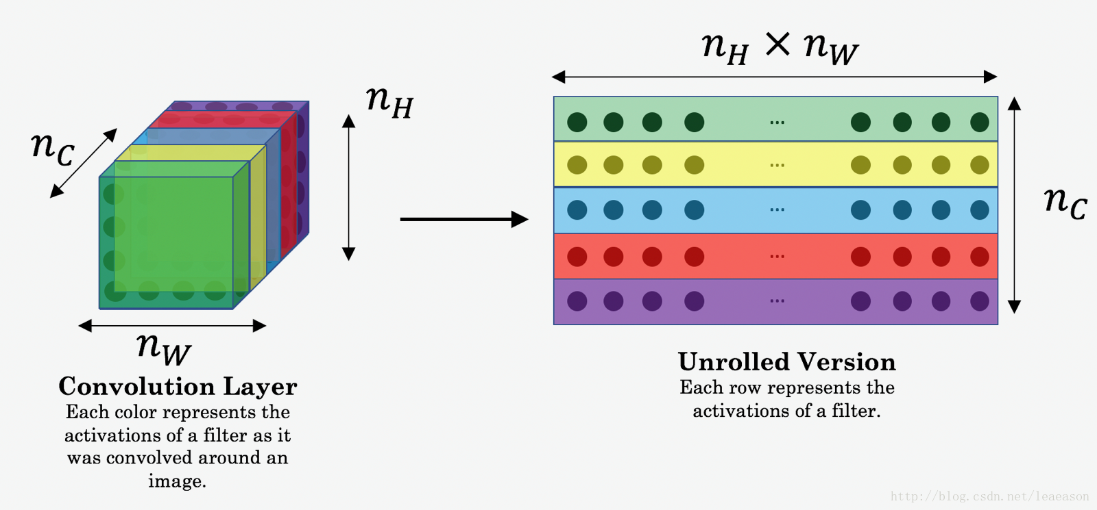
# Reshape the images to have them of shape (n_C, n_H*n_W) (≈2 lines)
a_S = tf.reshape(a_S,shape=(n_H*n_W,n_C))
a_G = tf.reshape(a_G,shape=(n_H*n_W,n_C))
# Computing gram_matrices for both images S and G (≈2 lines)
GS = gram_matrix(tf.transpose(a_S))
GG = gram_matrix(tf.transpose(a_G))
# Computing the loss (≈1 line)
J_style_layer = tf.reduce_sum(tf.square(tf.subtract(GS,GG)))/(4*(n_C*n_C)*(n_W * n_H) * (n_W * n_H))
### END CODE HERE ###
return J_style_layertf.reset_default_graph()
with tf.Session() as test:
tf.set_random_seed(1)
a_S = tf.random_normal([1, 4, 4, 3], mean=1, stddev=4)
a_G = tf.random_normal([1, 4, 4, 3], mean=1, stddev=4)
J_style_layer = compute_layer_style_cost(a_S, a_G)
print("J_style_layer = " + str(J_style_layer.eval()))J_style_layer = 9.19028
3.2.3 Pesas de estilo
def compute_style_cost(model, STYLE_LAYERS):
    """
    Computes the overall style cost from several chosen layers

    Arguments:
    model -- our tensorflow model
    STYLE_LAYERS -- A python list containing:
                        - the names of the layers we would like to extract style from
                        - a coefficient for each of them

    Returns:
    J_style -- tensor representing a scalar value, style cost defined above by equation (2)
    """

    # initialize the overall style cost
    J_style = 0

    for layer_name, coeff in STYLE_LAYERS:

        # Select the output tensor of the currently selected layer
        out = model[layer_name]

        # Set a_S to be the hidden layer activation from the layer we have selected, by running the session on out
        a_S = sess.run(out)

        # Set a_G to be the hidden layer activation from same layer. Here, a_G references model[layer_name]
        # and isn't evaluated yet. Later in the code, we'll assign the image G as the model input, so that
        # when we run the session, this will be the activations drawn from the appropriate layer, with G as input.
        a_G = out

        # Compute style_cost for the current layer
        J_style_layer = compute_layer_style_cost(a_S, a_G)

        # Add coeff * J_style_layer of this layer to overall style cost
        J_style += coeff * J_style_layer

    return J_style
3.3 - Definición del costo total para optimizar
# GRADED FUNCTION: total_cost

def total_cost(J_content, J_style, alpha = 10, beta = 40):
    """
    Computes the total cost function

    Arguments:
    J_content -- content cost coded above
    J_style -- style cost coded above
    alpha -- hyperparameter weighting the importance of the content cost
    beta -- hyperparameter weighting the importance of the style cost

    Returns:
    J -- total cost as defined by the formula above.
    """

    ### START CODE HERE ### (≈1 line)
    J = alpha*J_content+beta*J_style
    ### END CODE HERE ###

return Jtf.reset_default_graph()
with tf.Session() as test:
np.random.seed(3)
J_content = np.random.randn()
J_style = np.random.randn()
J = total_cost(J_content, J_style)
print("J = " + str(J))4 - Resolviendo el problema de optimización
J = total_cost(J_content,J_style,10,40)
# define optimizer (1 line)
optimizer = tf.train.AdamOptimizer(2.0)

# define train_step (1 line)
train_step = optimizer.minimize(J)
def model_nn(sess, input_image, num_iterations = 200):
# Initialize global variables (you need to run the session on the initializer)
### START CODE HERE ### (1 line)
sess.run(tf.global_variables_initializer())
### END CODE HERE ###
# Run the noisy input image (initial generated image) through the model. Use assign().
### START CODE HERE ### (1 line)
generated_image=sess.run(model['input'].assign(input_image))
### END CODE HERE ###
for i in range(num_iterations):
# Run the session on the train_step to minimize the total cost
### START CODE HERE ### (1 line)
sess.run(train_step)
### END CODE HERE ###
# Compute the generated image by running the session on the current model['input']
### START CODE HERE ### (1 line)
generated_image=sess.run(model['input'])
### END CODE HERE ###
# Print every 20 iteration.
if i%20 == 0:
Jt, Jc, Js = sess.run([J, J_content, J_style])
print("Iteration " + str(i) + " :")
print("total cost = " + str(Jt))
print("content cost = " + str(Jc))
print("style cost = " + str(Js))
# save current generated image in the "/output" directory
save_image("output/" + str(i) + ".png", generated_image)
# save last generated image
save_image('output/generated_image.jpg', generated_image)
return generated_imageImágenes después de 20 iteraciones: Imágenes después de
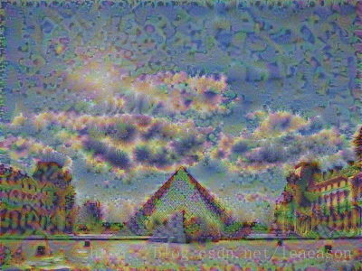
180 iteraciones: Imágenes después de
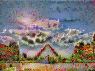
200 iteraciones: