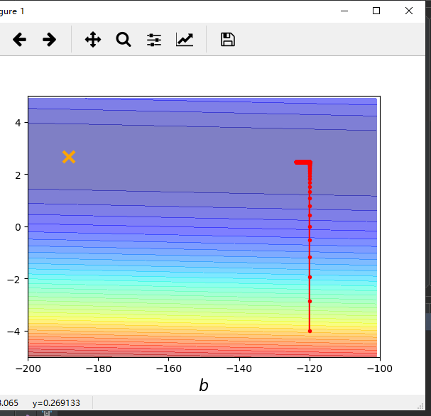
Import numpy AS NP
 Import matplotlib.pyplot AS PLT

x_data = [338,333,328,207,226,25,179,60,208,606 ]
y_data = [640,633,619,393,428,27,193,66,226,1591 ]


# generated number from -200 to -100, -100 does not include the
# X-axis
x = np.arange (-200, -100,1 )
 # Y-axis
Y = np.arange (-5,5,0.1 )
 # store corresponding error
the Z = np.zeros ((len (X), len (Y)) )
 # X tiled horizontally to X, y tile Vertically to the Y
# X-, np.meshgrid the Y = (X, Y)
for I in Range (len (X)):
     for J in Range (len (Y)):
        b= X [I]
        W = Y [J]
         # rows calculating error
        the Z [J] [I] = 0
         # error and
        for n- in Range (len (x_data)):
            the Z [J] [I] = the Z [ J] [I] + (y_data [n-] - B - * x_data W [n-]) ** 2
         # normalizing
        the Z [J] [I] = the Z [J] [I] / len (x_data)


# Y W * X + B =
B = -120
W = -4
LR = 0.0000001
Iteration = 100000

b_history = [B]
w_history = [W]

for I in Range (Iteration):
    b_grad= 0.0
    w_grad = 0.0

    for n in range(len(x_data)):
        b_grad = b_grad - 2.0*(y_data[n] - b - w*x_data[n])*1.0
        w_grad = w_grad - 2.0 * (y_data[n] - b - w * x_data[n]) * x_data[n]

    b = b - lr * b_grad
    w = w - lr * w_grad

    b_history.append(b)
    w_history.append(w)

plt.contourf(x, y, Z, 50, alpha=0.5, cmap=plt.get_cmap('jet'))
plt.plot([-188.4],[2.67],'x',ms=12,markeredgewidth=3,color='orange')
plt.plot(b_history,w_history,'o-',ms = 3,lw = 1.5,color = 'red')
plt.xlim(-200,-100)
plt.ylim(-5,5)
plt.xlabel(r'$b$',fontsize=16)
plt.ylabel(r'$w$',fontsize=16)
plt.show()