Analyze simple time series from the perspective of signal processing and directly perform various spectral analysis (spectrum, envelope spectrum, squared envelope spectrum, power spectrum, cepstrum, etc.), such as some simple rotating machinery vibration time series signals

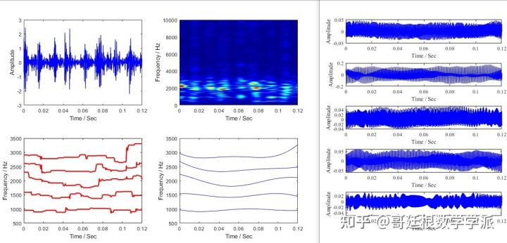
If the spectrum is difficult to analyze, you can analyze the time spectrum of the time series as shown in the figure below

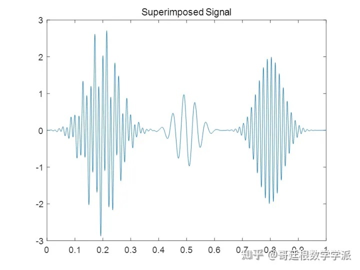
Give a simple example of an analog signal: t = 0:1/2000:1-1/2000; dt = 1/2000; x1 = sin(50*pi*t).*exp(-50*pi*( t -0.2).^2); x2 = sin(50*pi*t).*exp(-100*pi*(t-0.5).^2); x3 = 2*cos(140*pi*t). *exp(-50*pi*(t-0.2).^2); x4 = 2*sin(140*pi*t).*exp(-80*pi*(t-0.8).^2); x = x1+x2+x3+x4 ; figure; plot(t,x) title('Superimposed Signal')
Its spectrum during continuous wavelet transform is as follows

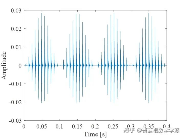
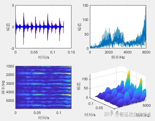
A simulated bearing inner ring fault vibration signal with obvious periodicity
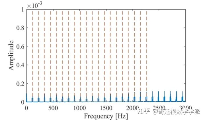
The corresponding spectrum is as follows. The red dotted line represents the fault characteristic frequency and the corresponding frequency multiplier.
The envelope spectrum is as follows

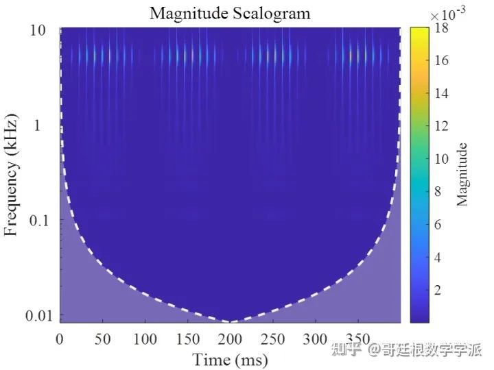
Looking at the corresponding CWT time spectrum, it is obvious that the impact
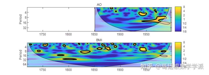
You can also try wavelet coherence and cross wavelet analysis. Wavelet coherence and cross wavelet can well reflect the "correlation" between changes in two different time series. Wavelet coherence analysis generally reflects the consistency of the periodic "changing trends" between sequences, but does not directly reflect the intensity relationship of the changing periods; cross wavelet analysis generally reflects the intensity of the "shared period" between sequences.


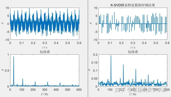
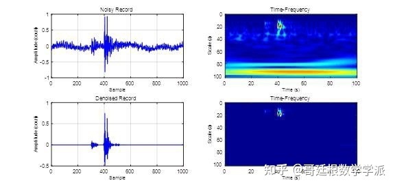
In addition, if the time-frequency spectrum line energy diverges and the time-frequency ridges are blurred, you can also try algorithms such as synchronous compression. Time Series Signal Processing Series - Synchronous Compression Transformation Based on Python - Articles from the Göttingen School of Mathematics - Zhihu Time Series Signal processing series - Synchronous compression transformation based on Python - Zhihu When the noise in the time series signal is large, in order to facilitate periodic analysis, it is inevitable to perform noise reduction pre-processing such as K-SVD noise reduction
Spline frame noise reduction
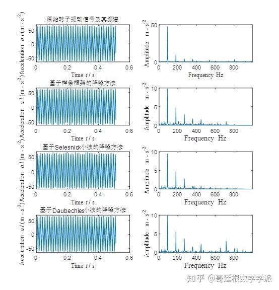
Morlet wavelet noise reduction

When the time series to be analyzed is too complex, it may be necessary to introduce modal decomposition (multi-resolution analysis), such as wavelet decomposition, empirical mode decomposition and its variants, variational mode decomposition, empirical wavelet transform, local mean decomposition , Symple geometric mode decomposition, various adaptive decomposition algorithms for time series decomposition based on wavelet ridges


Many students are interested in time series processing of various modal decomposition methods. Let me just talk about it. In fact, time series are usually composed of multiple components with physical meaning. In many cases, in order to study signals more easily, we It is desirable to study one or more of these components individually on the same time scale as the original data. Ideally, we want these multiple components decomposed by MRA to be physically meaningful and easily interpretable. Multi-resolution analysis MRA is usually associated with wavelets or wavelet packets, but modal decomposition methods such as empirical mode decomposition EMD, variational mode decomposition VMD, etc. can also constitute MRA. First, give a simple synthetic signal. The signal is sampled at a frequency of 1000Hz for 1 second. Fs = 1e3; t = 0:1/Fs:1-1/Fs; comp1 = cos(2*pi*200*t).*(t>0.7); comp2 = cos(2*pi*60*t) .*(t>=0.1 & t<0.3); trend = sin(2*pi*1/2*t); rng default wgnNoise = 0.4*randn(size(t)); x = comp1+comp2+trend+ wgnNoise; plot(t,x) xlabel('Seconds') ylabel('Amplitude') title('Synthetic Signal')
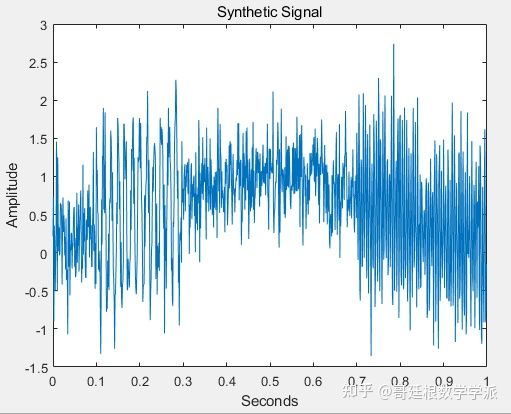
The signal consists of 3 main components: a time local oscillation component with a frequency of 60 Hz, a time local oscillation component with a frequency of 200 Hz, and a trend component. The trend component is a sinusoidal curve with a frequency of 0.5Hz. The 60Hz oscillation component occurs between 0.1 and 0.3 seconds, while the 200Hz oscillation component occurs between 0.7 and 1 second. However, these components cannot be distinguished from the time domain waveform, so frequency domain transformation is performed. xdft = fft(x); N = numel(x); xdft = xdft(1:numel(xdft)/2+1); freq = 0:Fs/N:Fs/2; plot(freq,20*log10( abs(xdft))) xlabel('Cycles/second') ylabel('dB') grid on
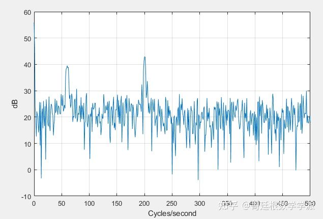
The frequency of the oscillating components can be more easily discerned from the frequency, but the temporal locality signal is lost. To simultaneously locate time and frequency information, continuous wavelet transform is used for analysis.

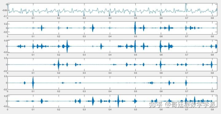
From the CWT time spectrum diagram, the time range of the 60Hz and 200Hz components can be seen, but no trend component is found. In order to isolate the components of the signal and analyze them individually, multi-resolution analysis is next used to perform correlation operations directly in the time domain. Multi-resolution analysis narrows the scope of analysis by dividing the signal into components of different resolutions. Extracting signal components of different resolutions is equivalent to decomposing the changes in the data on different time scales, or equivalently performing analysis on different frequency bands. First, the maximum overlap discrete wavelet transform, a variant of the discrete wavelet transform, is used to conduct multi-resolution analysis of the signal, with the number of decomposition layers being 8. For related content on maximum overlap discrete wavelet transform, please check the following literature.

The 8-layer multi-resolution analysis of maximum overlap discrete wavelet transform is decomposed as follows:

If you look from top to bottom, you will see that the decomposed components become smoother and smoother, that is, the component frequencies are getting lower and lower. Recall that the original signal contains 3 main components, a high-frequency oscillation component at 200 Hz, a low-frequency oscillation component at 60 Hz, and a trend component, all of which are destroyed by additive noise. It can be seen from the D2 plot that the time-localized high-frequency components are decomposed, while the following two plots contain lower frequency oscillatory components, which is an important aspect of multi-resolution analysis. Finally, the S8 subfigure contains Trend term components. In addition to wavelet multi-resolution analysis, empirical mode decomposition (EMD) is a so-called data-adaptive multi-resolution technique. EMD recursively extracts different resolution components from the data without using fixed basis functions. There is a vast amount of literature related to EMD, so I won’t go into details. The multi-resolution analysis decomposition of EMD is as follows:

Although the number of MRA decomposition components is different, EMD MRA and wavelet MRA will produce similar signal waveforms. In EMD MRA decomposition, the high-frequency oscillation component is located in the first intrinsic mode function (IMF1), and the low-frequency oscillation component is mainly Located in IMF2 and IMF3, the trend term component in IMF6 is very similar to the trend component extracted by wavelet technology. Another technique for adaptive multi-resolution analysis is variational mode decomposition (VMD). VMD extracts intrinsic mode functions or oscillation modes from the signal and does not use fixed basis functions for analysis. EMD is recursive in the time domain to gradually extract low-frequency IMF components, while VMD first identifies signal peaks in the frequency domain and extracts all modes simultaneously. The relevant literature is as follows: Dragomiretskiy, Konstantin, and Dominique Zosso. “Variational Mode Decomposition.” IEEE Transactions on Signal Processing 62, no. 3 (February 2014): 531–44. https://doi.org/10.1109/TSP.2013.2288675 . The multi-resolution analysis decomposition of VMD is as follows:
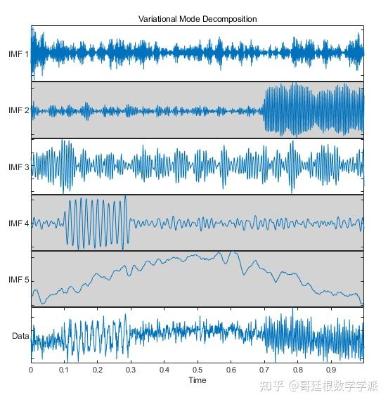
As can be seen from the above figure, similar to wavelet and EMD, VMD basically separates the three components. There is also a data adaptive multi-resolution analysis technology: Empirical Wavelet Transform (EWT). EWT constructs a Meye wavelet based on the frequency of the analyzed signal and then performs adaptive wavelet. I have written about EWT before: Empirical Wavelet Transform in Signal Processing and Bearing Failures Application in diagnosis - Article by Göttingen School of Mathematics - Zhihu https://zhuanlan.zhihu.com/p/53 The multi-resolution analysis decomposition of EWT is as follows:
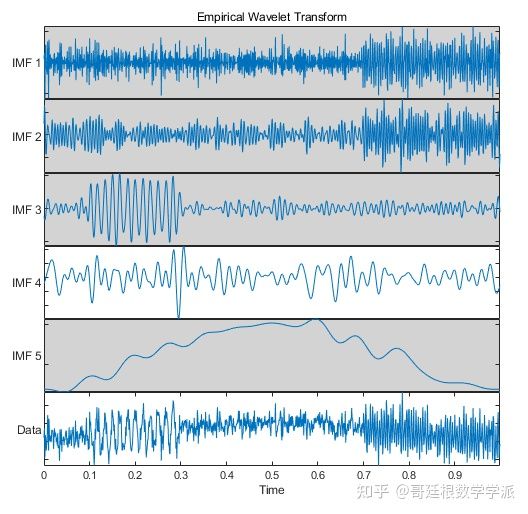
Similar to the previous EMD and wavelet MRA, EWT decomposes the relevant oscillation components. The filters used to perform the analysis and their passband information are as follows:

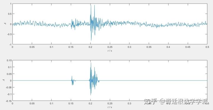
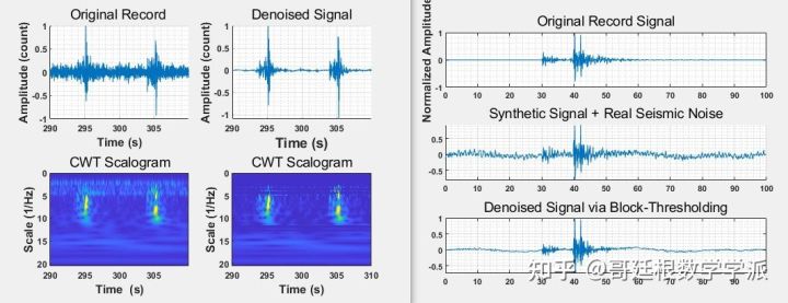
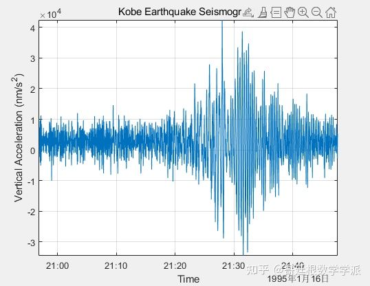
Consider below a Kobe earthquake signal , recorded at the University of Tasmania in Hobart, Australia, on January 16, 1995 , starting at 20:56:51 (GMT) and lasting for 51 minutes at 1 second intervals. figure plot(T,kobe) title('Kobe Earthquake Seismograph') ylabel('Vertical Acceleration (nm/s^2)') xlabel('Time') axis tight grid on
Taking the maximum overlap discrete wavelet transform as an example, its 8-layer MRA is decomposed as follows:

From the D4 and D5 subfigures, we can see the primary and delayed secondary wave components. The components in the seismic wave propagate at different speeds, and the primary wave propagates faster than the secondary (shear) wave. The purpose of decomposing a signal into several components is usually to remove certain components to reduce the impact on signal analysis. The key to MRA technology is the ability to reconstruct the original signal, as follows:

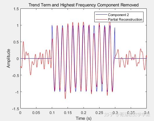
The maximum reconstruction error for each method is about 10^(-12) or less, indicating that they can reconstruct the signal perfectly. In many studies, we are not interested in the trend term. Since the trend term is generally located in the last MRA decomposition component, we only need to remove this component and then reconstruct it.

In addition, delete the first MRA decomposition component (it seems to be mainly noise)
In the previous section, we deleted the trend term. However, in many applications, the trend term may be our main research part, so we visualize the trend term components extracted by several MRA methods.

According to the above analysis, wavelet MRA technology can extract the trend term more smoothly and most accurately. EMD extracts a smooth trend term, but it is offset relative to the true trend amplitude, while VMD seems to be more biased than wavelet and EMD. Extract the oscillation components. In the previous examples, the role of multiresolution analysis in detecting oscillatory components and overall trends in the data was emphasized, however MRA can also locate and detect transient components in the signal. To illustrate this point, using U.S. real gross domestic product (GDP) data from the first quarter of 1947 to the fourth quarter of 2011, the vertical black line marks the beginning of the “Great Moderation”, marking the beginning of the mid-1980s. Periods of reduced macroeconomic volatility are difficult to discern from the raw data.

See some code links in the comment area. Download more bread. The content includes modern signal processing, machine learning, deep learning, fault diagnosis, etc.