We had more than a dozen articles before that described the basic theory of EMD algorithm, the meaning of IMF, the MATLAB implementation method of EMD, the theory and code implementation of EEMD , CEEMD , CEEMDAN , VMD , ICEEMDAN , LMD , EWT , SWT, and also talked about HHT algorithm theory and its code implementation .
The previous article introduced the variance contribution rate, average period, and correlation coefficient of the IMF component . Today, I will talk about the commonly used and easy-to-use IMF processing methods.
1. Restructuring of the IMF
Many students asked how to do IMF reconstruction. Signal reconstruction is indeed an important method for post-processing of EMD methods. Refactoring usually faces two problems:
(1) How to implement the refactoring operation?
(2) Which components to choose for reconstruction?
First answer the first question (1) . In fact, the so-called "refactoring" is simply understood as "addition". For example, if you want to reconstruct the 1st, 3rd, and 5th IMF components, just add the corresponding components.
Specifically in the code implementation, if you use the series of codes decomposed by "like EMD" in this column, the author has unified the decomposition algorithm: the decomposed IMF components are arranged along the row vector, that is, the IMF's The dimension is (m,n), where m represents the number of IMF components (including res), and n represents the data length.
At this time, the reconstruction of IMF1, 3, and 5 can be written as:
IMFnew = imf(1,:)+imf(3,:)+imf(5,:);
For the second question, it is relatively complicated. For the screening criteria that need to be selected, it is recommended that students refer to the usual practice of related papers in the research field, because the EMD method has a wide range of applications, and the methods used for different purposes will be different.
However, the following is a relatively general refactoring method.
2. Discrimination and reconstruction of high-frequency, low-frequency, and trend item components
The trend item is the res component, which does not require additional effort to distinguish.
Our main concern is how to distinguish between high frequency and low frequency components.
The criteria used here are as follows [1] :
Record IMF1 as index 1, IMF1+IMF2 as index 2, and so on, the sum of the first i IMFs is index i, calculate the mean value of index 1 to index 7, and perform t-test whether 0 test. ( Some papers directly use each IMF component as the corresponding index, and this paper uses each IMF component as the calculation method of the corresponding index )
Why use whether it is significantly different from 0 as the boundary between high and low frequencies? When we talked about EMD decomposition before, we said that the IMF component must satisfy the local symmetry of the upper and lower envelopes with respect to the time axis. For high-frequency IMF components , the upper and lower envelopes are basically obtained by connecting many signal peak points, so the symmetry of the envelope means that the IMF component data is basically symmetrical, and the data mean value approaches 0; for low-frequency IMF component , the signal period is large, the envelope is obtained by a small amount of peak interpolation, and the envelope trend deviates greatly from the original signal trend, so when the envelope is symmetrical, the signal components are often asymmetrical, and even deviate far away. At this time, the IMF component is natural It is difficult to guarantee that the mean is 0.
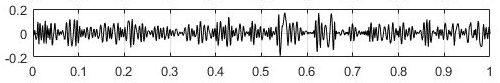
The high-frequency component obtained by decomposing a certain signal

The low frequency component obtained by decomposing a certain signal
Observing the two diagrams of high-frequency components and low-frequency components above, it should be easier to understand that the mean value of high-frequency components tends to 0, and the low-frequency components are less likely to approach 0.
For example, let’s take the historical data of crude oil futures prices from 2012 to 2020 in the previous article as an example, and first perform EEMD decomposition:

Install the above ideas to carry out t-test, and find that the index 5 is significantly different from 0, then IMF1-4 represent high-frequency components, and IMF5-10 represent low-frequency components.
At this time, we reconstruct the high-frequency component and low-frequency component separately to obtain the high-frequency and low-frequency features of the data.
We draw high-frequency features, low-frequency features, trend items and original signals on the same graph:
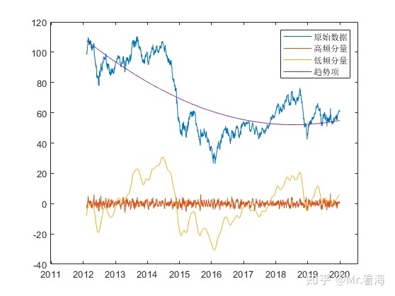
The result is still beautiful.
Fourth, MATLAB code implementation
According to the convention, the above functions are encapsulated into a function file that is convenient to call. I named it the imfHLdif function. The function description is as follows:
function [HighCom,LowCom,TrCom,HighIdx,LowIdx]=imfHLdif(data,imf,figflag)
%% 根据重构算法将分解得出的IMF进行高低频的区分
% 参考《基于EEMD模型的中国碳市场价格形成机制研究》
% 该方法将IMF1记为指标1,IMF1+IMF2为指标2,以此类推,
% 前i个IMF的和加成为指标i,并对该均值是否显著区别于0进行t检验。
% 输入:
% data:分解前的原始数据
% imf:经过模态分解方法得到的分量,每一行为一个分量
% figflag:设置是否画图的参数,'on'为画图,'off'为不画图
% 输出:
% HighCom:重构后的高频分量
% LowCom:重构后的低频分量
% TrCom:趋势项
% HighIdx:高频分量对索引
% LowIdx:低频分量对索引
All it takes is one line of code to call:
[HighCom,LowCom,TrCom,HighIdx,LowIdx]=imfHLdif(data,imf,'on');
The discrimination and reconstruction of high and low frequency components, the export of trend items, and the drawing of reconstructed images (the picture above) can all be realized.
The above test cases and wrapper functions, including the toolbox, can be obtained from the following link:
There are also programs related to EMD, EEMD, CEEMD, CEEMDAN, ICEEMDAN, VMD and HHT. Programming is not easy, thank you for your support~ For the introduction of EMD, EEMD, CEEMD, VMD and HHT, you can see here:
Mr. Watching the Sea: EMD-like "Signal Decomposition Method" and MATLAB Implementation (Part 4)——VMD
Mr. Watching the Sea: EMD-like "Signal Decomposition Method" and MATLAB Implementation (Part 7)——EWT
refer to
- ^ Qi Shaozhou, Zhao Xin, Tan Xiujie. Research on the price formation mechanism of China's carbon market based on EEMD model [J]. Journal of Wuhan University: Philosophy and Social Science Edition, 2015(4):56-65.