The difference between logistic regression and linear regression:
(1) The function fitting of linear regression is used for numerical prediction, and logistic regression is a binary classification algorithm for classification;
(2) Linear regression model:
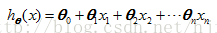
Logistic regression model:
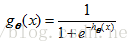
That is to say, logistic regression is actually based on linear regression, and an excitation function mapping is added. Because logistic regression is a binary classification algorithm, there are only two values for training data, 1 and 0 , representing two classifications. When used for prediction classification, if the input value is greater than 0.5 , it will be classified as class 1 , otherwise are classified as category 0 . Therefore, the training data needs to satisfy the following probability formula:
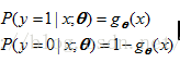
Our training process is to train the parameter θ, so that the above two probabilities are as 1 as possible;
(3) The commonly used cost function of linear regression is defined as:
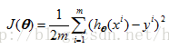
The logistic regression cost function is :
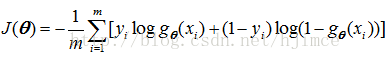
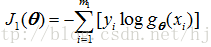
In fact, the above formula can be written separately. For class 1 , the total cost function is: :
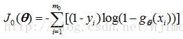
For class 0 , the total cost function is:
therefore:
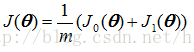
Our purpose is to minimize the value of the cost function J( θ ) and make it as close to 0 as possible .
(4) Gradient descent method to solve.
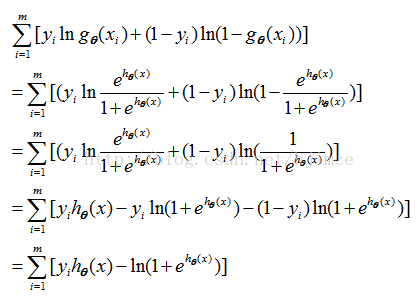
Cost function simplification:
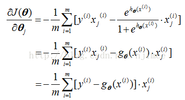
OK , after the simplification of the formula is completed, the partial derivative is then calculated:
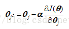
After the derivation is completed, the next step is to directly use the formula of the gradient descent method:
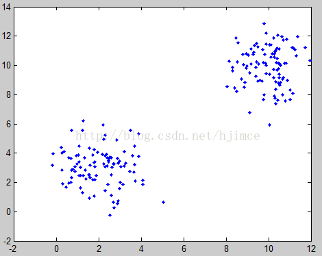
Then write the matlab code and train it. Only after you have written the code yourself can you be really familiar with this algorithm:
close all;
clear;
clc;
% Generate test data
mu = [2 3];% test data 1
SIGMA = [1 0; 0 2];
r1 = mvnrnd(mu,SIGMA,100);
plot(r1(:,1),r1(:,2),'.');
hold on;
mu = [10 10];% test data 2
SIGMA = [ 1 0; 0 2];
r2 = mvnrnd (in, SIGMA, 100);
plot (r2 (:, 1), r2 (:, 2), '.');
data(:,2:3)=[r1;r2];
data(:,1)=1;

% training data label
flag=[ones(100,1);zeros(100,1)];
[m,n]=size(data);
w=zeros(n,1);
% gradient descent
sigma=0.05;
i=1;
while i<10000
   for j=1:n
    % Calculate the excitation function value first
    pp=data*w;
    pp=exp(-data*w);
    gx=1./(1+exp(-data*w));
    % Calculate partial derivative value
     r=-1/m*sum((flag-gx).*data(:,j));
     w(j)=w(j)-sigma*r;
   end
   i=i+1;
end
% draw the classification results
figure(2);
hold on;
for i=1:m
    if gx(i)>0.5
        plot(data(i,2),data(i,3),'.b');
    else
        plot(data(i,2),data(i,3),'.y');
    end
end
% draw the decision boundary line
w(2)=w(2)/sqrt(w(2)*w(2)+w(3)*w(3));
w(3)=w(3)/sqrt(w(2)*w(2)+w(3)*w(3));
line([4,9],[(4*w(2)+w(1))/(-w(3)),(9*w(2)+w(1))/(-w(3))]);
Original image classification result: