SVM-based classification of breast cancer datasets

1. About the author

Che Chenjie, female, School of Electronic Information, Xi'an Polytechnic University, 21st-level graduate student
Research direction: Machine Vision and Artificial Intelligence
Email: [email protected]

Liu Shuaibo, male, School of Electronic Information, Xi'an Polytechnic University, 2021 graduate student, Zhang Hongwei Artificial Intelligence Research Group
Research direction: Machine Vision and Artificial Intelligence
Email: [email protected]

2. Introduction to SVM algorithm

2.1 SVM algorithm

Support vector machines (SVM) is a binary classification model. The purpose of SVM is to find a line that "best" distinguishes these two types of points, so that if there are new points in the future, this line will also Can make a good classification, which is illustrated in two dimensions. In high-dimensional space, we want to distinguish two types of sample data, we need to find a hyperplane to distinguish the two types of sample data. SVM is suitable for small and medium data samples, nonlinear, high-dimensional classification problems.
"Three-eight lines" can be seen as a visual interpretation of SVM in two-dimensional space. It conveys the following important information:
(1) It is a straight line (linear function);
(2) The desktop can be divided into two parts , belong to you and me respectively (with a classification function, it is a binary classification);
(3) It is located in the middle of the desk and does not favor any one party (focusing on the principle of fairness can ensure that the interests of both parties are maximized).
The above three points are the central idea of ​​SVM algorithm.

2.2 Understanding and Analysis of SVM Algorithm

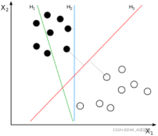
The SVM will find the partitioning hyperplane that can distinguish the two classes and maximize the margin. If the hyperplane is better divided, the local perturbation of the sample will have the least impact on it, the classification results will be the most robust, and the generalization ability to unseen examples will be the strongest. As can be seen from the figure below, H1 is linearly inseparable, and H2 and H3 are linearly separable. At this time, we use the principle of the largest interval to select H3 as the hyperplane that distinguishes the two types of sample points in the following figure.

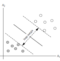
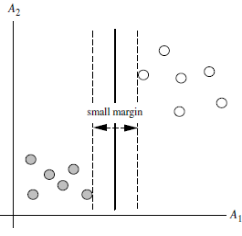
As can be seen from the figure below, the distances from the points on the dotted line to the dividing hyperplane are the same. In fact, only these points jointly determine the position of the hyperplane, so they are called "support vectors". This is where "support vector machines" come from.


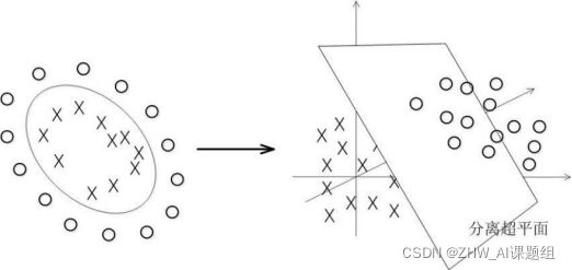
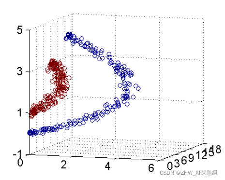
In fact, most of the time the data is not linearly separable, and a hyperplane that satisfies such a condition does not exist at all. For the nonlinear case, the processing method of SVM is to select a kernel function κ(⋅,⋅), by mapping the data to the high-dimensional space, and finally construct the optimal separation hyperplane in the high-dimensional feature space, so as to put the plane on the plane. Separation of non-linear data that is not inherently good. As shown in the figure, a bunch of data cannot be divided in two-dimensional space, so it is mapped to three-dimensional space.

The purpose of the kernel function is to classify the data. This topic uses linear kernel, polynomial kernel, Gaussian kernel (rbf) and sigmoid. The kernel function is tested and explained.
We use a moving picture to show the above expression:

3. Introduction to the Breast Cancer Dataset

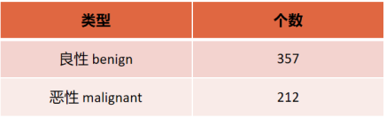
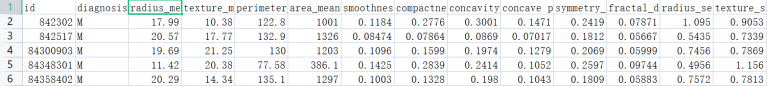
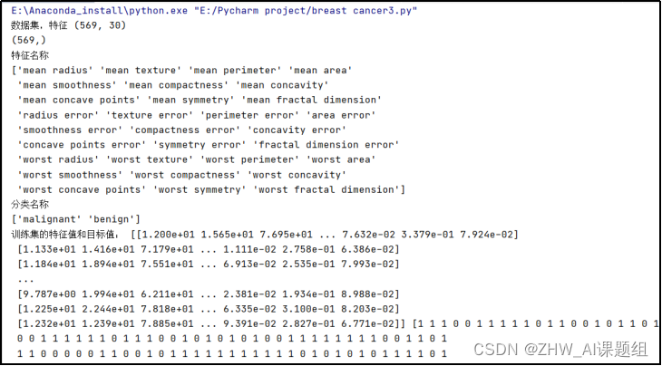
This topic uses the Breast Cancer Wisconsin (Diagnostic) Data Set (Wisconsin Breast Cancer (Diagnostic) Data Set), which has a total of 569 samples and 30 features (10 mean, 10 standard deviation, 10 maximum value), the label is binary classification. The figure below shows the breast cancer dataset and a detailed description of the 30 features. The following are the specific types and numbers of binary labels and some screenshots of the breast cancer dataset: The


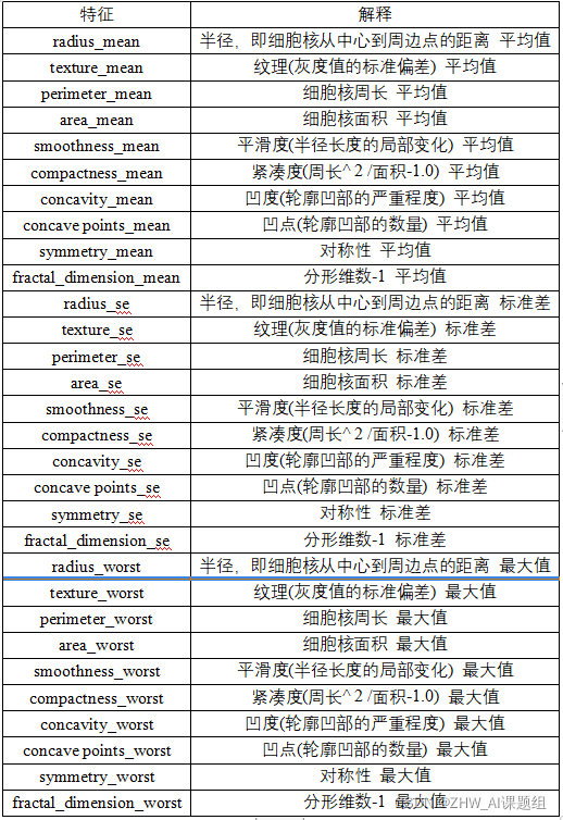
30 features and their corresponding explanations are as follows:

4. SVM-based breast cancer dataset classification experiment

4.1 Import the required packages

from sklearn.datasets import load_breast_cancer
from sklearn.svm import SVC
from sklearn.model_selection import train_test_split
import matplotlib.pyplot as plt
import numpy as np

4.2 Importing breast cancer dataset

cancers = load_breast_cancer() #下载乳腺癌数据集
X = cancers.data  #获取特征值
Y = cancers.target  #获取标签

4.3 Output data sets, features and other data

print("数据集，特征"，X.shape)  #查看特征形状
print(Y.shape)  #查看标签形状
#print(X)#输出特征值
#print(Y)#输出特征值
#print(cancers.DESCR)   #查看数据集描述
print('特征名称')#输出特征名称 
print(cancers.feature_names)  # 特征名
print('分类名称')#输出分类名称 
print(cancers.target_names)  # 标签类别名
# 注意返回值： 训练集train，x_train，y_train，测试集test，x_test，y_test
# x_train为训练集的特征值，y_train为训练集的目标值，x_test为测试集的特征值，y_test为测试集的目标值
# 注意，接收参数的顺序固定
# 训练集占80%，测试集占20%

x_train, x_test, y_train, y_test = train_test_split(X, Y, test_size=0.2)
print('训练集的特征值和目标值：', x_train, y_train) 
#输出训练集的特征值和目标值 
    print('测试集的特征值和目标值：', x_test, y_test)
#输出测试集的特征值和目标值
#print(cancers.keys())

#可以根据自己写代码的习惯输出上述参数

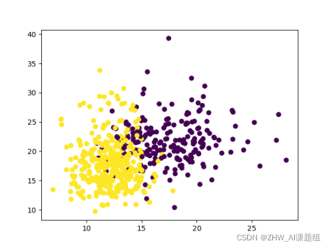
4.4 Visualizing the Breast Cancer Dataset

np.unique(Y)  # 查看label都由哪些分类
plt.scatter(X[:, 0], X[:, 1], c=Y)
plt.show() #显示图像

4.5 Modeling training

#下面是四种核函数的建模训练

# 线性核
model_linear = SVC(C=1.0, kernel='linear')

# 多项式核
#degree表示使用的多项式的阶数
model_poly = SVC(C=1.0, kernel='poly', degree=3)

# 高斯核(RBF核)
#gamma是核函数的一个参数，gamma的值会影响测试精度
model_rbf = SVC(C=1.0, kernel='rbf', gamma=0.1)

# sigmoid核
gammalist=[]  #把gammalist定义为一个数组
score_test=[]  #把score_test定义为一个数组
gamma_dis=np.logspace(-100,-5,50)
#gamma_dis从10-100到10-5平均取50个点
for j in gamma_dis:
    model_sigmoid = SVC(kernel='sigmoid', gamma=j,cache_size=5000).fit(x_train, y_train)
    gammalist.append(j)
    score_test.append(model_sigmoid.score(x_test, y_test))
#找出最优gammalist值
print("分数--------------------",score_test)
print("测试最大分数， 
gammalist",max(score_test),gamma_dis[score_test.index(max(score_test))])
plt.plot(gammalist,score_test) #横轴为gammalist纵轴为score_test
plt.show()#显示图片

The output results are as follows:


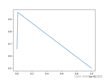
From the output data and pictures, we can see that when gamma = 1.1513953993264481e-07, the test accuracy is the highest, which is 0.9298245614035088. When the test accuracy is the highest, we call the corresponding gamma value the optimal gamma value.

4.6 Output training scores and test scores

model_linear.fit(x_train, y_train)
train_score = model_linear.score(x_train, y_train)
test_score = model_linear.score(x_test, y_test)
print('train_score:{0}; test_score:{1}'.format(train_score, test_score))
#线性核函数输出训练精度和测试精度

model_poly.fit(x_train, y_train)
train_score = model_poly.score(x_train, y_train)
test_score = model_poly.score(x_test, y_tetrain_score = model_rbf.score(x_train, y_train)
test_score = model_rbf.scorst)
print('train_score:{0}; test_score:{1}'.format(train_score, test_score))
#多项式函数输出训练精度和测试精度

model_rbf.fit(x_train, y_train)
e(x_test, y_test)
print('train_score:{0}; test_score:{1}'.format(train_score, test_score))
#rbf(高斯核)函数输出训练精度和测试精度

model_sigmoid.fit(x_train, y_train)
train_score = model_sigmoid.score(x_train, y_train)
test_score = model_sigmoid.score(x_test, y_test)
print('train_score:{0}; test_score:{1}'.format(train_score, test_score))
#sigmoid函数输出训练精度和测试精度

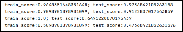
The output is as follows:

5 Conclusion

1. By comparison, the linear kernel (linear) and the polynomial kernel (poly) have higher test accuracy, while the Gaussian kernel (rbf) and the sigmoid kernel have lower test accuracy. Therefore, the results obtained by using the linear kernel and polynomial kernel test in this topic are ideal (we follow-up You can also modify the code yourself to improve the accuracy of the rbf kernel function and the sigmoid kernel function);
2. The test accuracy of the Gaussian kernel is 1;
3. In the sigmoid kernel function, the value of gamma has an impact on the test accuracy. And when
   gamma=1.1513953993264481e-07, the test accuracy is the highest, which is 0.9298245614035088
   5. Reference link The
   breast cancer dataset comes from
   https://pan.baidu.com/s/1DN4AlRzDkmBSZlnk8dY15g Extraction code: i6u6
   blog reference link:
   https://blog .csdn.net/qq_42363032/article/details/107210881