Linear regression
In statistics, linear regression is a linear method of modeling the relationship between a scalar response and one or more explanatory variables (also called dependent variables and independent variables).
In recent years, linear linear regression has played an important role in the field of artificial intelligence and machine learning. Linear regression algorithm has become one of the basic algorithms of supervised machine learning because of its relatively simple and well-known characteristics. Interested readers can refer to deep learning materials. For example, Andrew Ng introduced linear regression from the perspective of deep learning (to page 7).
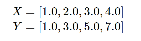
However, since this is not a deep learning course, we will solve this problem from a mathematical perspective. We start by learning a specific example and give the following data (in deep learning terms, these data are called training data):
Our goal is to generate a linear function :![]()
Make it fit the above data as close as possible, where the variables and the unknown variables. By "as close as possible", we use the least squares method, that is, we want to minimize the following expression:
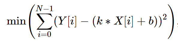 N is the length of X or Y
Now the next step is to solve equation (6) to calculate the sum of the values of the variables. We will use Z3 to accomplish this task, because Z3 also supports some nonlinear constraint solving.
Exercise 18: Read the code in the linear_regression.py Python file, you need to install the matplotlib package to run this code. You can install matplotlib via pip:
pip install matplotlibOr, you can install them through PyChram's preferences, just like we did in the software settings of homework 1. After setting the environment, complete the lr_training() method and use Z3 for linear regression.
import matplotlib.pyplot as plt
from z3 import *
from linear_regression_ml import sklearn_lr
class Todo(Exception):
def __init__(self, msg):
self.msg = msg
def __str__(self):
return self.msg
def __repr__(self):
return self.__str__()
################################################
# Linear Regression (from the SMT point of view)
# In statistics, linear regression is a linear approach to modelling
# the relationship between a scalar response and one or more explanatory
# variables (also known as dependent and independent variables).
# The case of one explanatory variable is called simple linear regression;
# for more than one, the process is called multiple linear regression.
# This term is distinct from multivariate linear regression, where multiple
# correlated dependent variables are predicted, rather than a single scalar variable.
# In recent years, linear Linear regression plays an important role in the
# field of artificial intelligence such as machine learning. The linear
# regression algorithm is one of the fundamental supervised machine-learning
# algorithms due to its relative simplicity and well-known properties.
# Interested readers can refer to the materials on deep learning,
# for instance, Andrew Ng gives a good introduction to linear regression
# from a deep learning point of view.
# However, as this is not a deep learning course, so we'll concentrate
# on the mathematical facet. And you should learn the background
# knowledge on linear regression by yourself.
# We start by studying one concrete example, given the following data
# (in machine learning terminology, these are called the training data):
xs = [1.0, 2.0, 3.0, 4.0]
ys = [1.0, 3.0, 5.0, 7.0]
# our goal is to produce a linear function:
# y = k*x + b
# such that it fits the above data as close as possible, where
# the variables "k" and "b" are unknown variables.
# By "as close as possible", we use a least square method, that is, we
# want to minimize the following expression:
# min(\sum_i (ys[i] - (k*xs[i]+b)^2) (1)
# Now the next step is to solve the equation (1) to calculate the values
# for the variables "k" and "b".
# The popular approach used extensively in deep learning is the
# gradient decedent algorithm, if you're interested in this algorithm,
# here is a good introduction from Andrew Ng (up to page 7):
# https://see.stanford.edu/materials/aimlcs229/cs229-notes1.pdf
# In the following, we'll discuss how to solve this problem using
# SMT technique from this course.
# Both "draw_points()" and "draw_line()" are drawing utility functions to
# draw points and straight line.
# You don't need to understand these code, and you can skip
# these two functions safely. If you are really interested,
# please refer to the manuals of matplotlib library.
# Input: xs and ys are the given data for the coordinates
# Output: draw these points [xs, ys], no explicit return values.
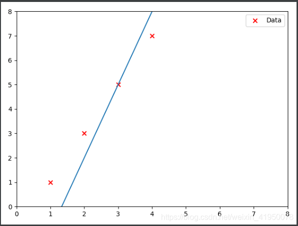
def draw_points(xs, ys):
plt.scatter(xs, ys, marker='x', color='red', s=40, label='Data')
plt.legend(loc='best')
plt.xlim(0, 8) # 设定绘图范围
plt.ylim(0, 8)
plt.savefig("./points.png")
plt.show()
# Input: a group of coordinates [xs, ys]
# k and b are coefficients
# Output: draw the coordinates [xs, ys], draw the line y=k*x+b
# no explicit return values
def draw_line(k, b, xs, ys):
new_ys = [(k*xs[i]+b) for i in range(len(xs))]
plt.scatter(xs, ys, marker='x', color='red', s=40, label='Data')
plt.plot(xs, new_ys)
plt.legend(loc='best')
plt.xlim(0, 8) # 设定绘图范围
plt.ylim(0, 8)
plt.savefig("./line.png")
plt.show()
# Arguments: xs, ys, the given data for these coordinates
# Return:
# 1. the solver checking result "res";
# 2. the k, if any;
# 3. the b, if any.
def lr_training(xs, ys):
# create two coefficients
k, b = Ints('k b')
# exercise 18: Use a least squares method
# (https://en.wikipedia.org/wiki/Least_squares)
# to generate the target expression which will be minimized
# Your code here:
# raise Todo("exercise 18: please fill in the missing code.")
exps = []
i = 0
for x in xs:
exps.append((ys[i] - k*x - b)*(ys[i] - k*x - b))
i = i+1
# print(exps)
# double check the expression is right,
# it should output:
#
# 0 +
# (1 - k*1 - b)*(1 - k*1 - b) +
# (3 - k*2 - b)*(3 - k*2 - b) +
# (5 - k*3 - b)*(5 - k*3 - b) +
# (7 - k*4 - b)*(7 - k*4 - b)
#
print("the target expression is: ")
print(sum(exps))
# create a solver
solver = Optimize()
# add some constraints into the solver, these are the feasible values
solver.add([k < 100, k > 0, b > -10, b < 10])
# tell the solver which expression to check
solver.minimize(sum(exps))
# kick the solver to perform checking
res = solver.check()
# return the result, if any
if res == sat:
model = solver.model()
kv = model[k]
bv = model[b]
return res, kv.as_long(), bv.as_long()
else:
return res, None, None
if __name__ == '__main__':
draw_points(xs, ys)
res, k, b = lr_training(xs, ys)
if res == sat:
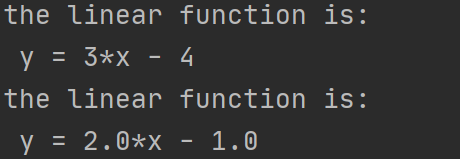
print(f"the linear function is:\n y = {k}*x {'+' if b >= 0 else '-'} {abs(b)}")
draw_line(k, b, xs, ys)
else:
print('\033[91m Training failed! \033[0m')
k, b = sklearn_lr(xs, ys)
print(f"the linear function is:\n y = {k}*x {'+' if b >= 0 else '-'} {abs(b)}")
# exercise 19: Compare the machine learning approach and the LP approach
# by trying some different training data. Do the two algorithms produce the same
# results? What conclusion you can draw from the result?
# Your code here:
Output result:
A popular method widely used in deep learning is the gradient decedent algorithm. If you are interested in this algorithm, Andrew Ng's note above contains a good introduction. In most cases, you don't need to reinvent the wheel. There are many effective machine learning libraries in Python, such as scikit-learn. You can use them directly to complete tasks.
Exercise 19: In the linear_regression_ml.py Python file, we provide a linear regression implementation based on the scikit-learn deep learning library. You don’t need to write any code, but you need to install the numpy and scikit-learn packages via pip:
pip install numpy
pip install scikit-learn
Or, you can install them via PyChram’s preferences, just like we did in the software settings of homework 1. Do that. After setting up the environment, you need to compare the machine learning method and the LP method (the method you achieved by trying some different training data in exercise 17). Do these two algorithms produce the same results? What conclusions can you draw from the results?
There is a question about this question and will be updated next week. = =
#中科大软院-hbj formalized course notes-Welcome to leave a message and exchange private messages
#随手点赞, I will be happier~~^_^