Introduction
Hey! I just finished a deep learning project a few hours ago, and now I want to share what I did. The goal of this challenge is to determine whether a person has pneumonia. If so, determine whether it is caused by bacteria or viruses. Well, I think this project should be called classification rather than detection.

In other words, this task will be a multi-classification problem, where the label names are: normal (normal), virus (virus) and bacteria (bacteria). To solve this problem, I will use CNN (Convolutional Neural Network), which has excellent image classification capabilities. Not only that, but here I also implemented image enhancement technology to improve model performance. By the way, I got 80% test data accuracy, which is very impressive for me.
The entire data set itself is about 1 GB in size, so downloading may take a while. Alternatively, we can directly create a Kaggle Notebook and encode the entire project there, so we don't even need to download any content. Next, if you browse the dataset folder, you will see that there are 3 subfolders, namely train, test and val.
Well, I think these folder names are self-explanatory. In addition, the data in the train folder includes 1341, 1345 and 2530 samples of normal, virus and bacteria categories respectively. I think this is all I have introduced, now let's get into the writing of the code!
Note: I put all the code used in this project at the end of this article.
Load modules and training images
When using a computer vision project, the first thing to do is to load all the necessary modules and the image data itself. I use the tqdm module to display the progress bar, and you will see why it is useful later.
The last thing I imported was the ImageDataGenerator from the Keras module. This module will help us implement image enhancement techniques during training.
import them
import cv2import pickleimport numpy as np
import matplotlib.pyplot as plt
import seaborn as sns
from tqdm import tqdm
from sklearn.preprocessing import OneHotEncoder
from sklearn.metrics import confusion_matrix
from keras.models import Model, load_model
from keras.layers import Dense, Input, Conv2D, MaxPool2D, Flatten
from keras.preprocessing.image import ImageDataGeneratornp.random.seed(22)
Next, I define two functions to load image data from each folder. At first glance, the two functions below may look exactly the same, but there are actually some differences in the lines shown in bold. This is done because the file name structure in the NORMAL and PNEUMONIA folders is slightly different. Despite the differences, the other processes performed by the two functions are basically the same.
First, adjust all images to 200 x 200 pixels.
This is important because the images in all folders have different sizes, and the neural network can only accept data with a fixed array size.
Next, basically all images are stored with 3 color channels, which is redundant for X-ray images. Therefore, my idea is to convert these color images to grayscale images.
# Do not forget to include the last slash
def load_normal(norm_path):    norm_files = np.array(os.listdir(norm_path))    norm_labels = np.array(['normal']*len(norm_files))
    norm_images = []    for image in tqdm(norm_files):
        image = cv2.imread(norm_path + image)        image = cv2.resize(image, dsize=(200,200))
        image = cv2.cvtColor(image, cv2.COLOR_BGR2GRAY)        norm_images.append(image)
    norm_images = np.array(norm_images)    return norm_images, norm_labels
def load_pneumonia(pneu_path):    pneu_files = np.array(os.listdir(pneu_path))    pneu_labels = np.array([pneu_file.split('_')[1] for pneu_file in pneu_files])
    pneu_images = []    for image in tqdm(pneu_files):
        image = cv2.imread(pneu_path + image)        image = cv2.resize(image, dsize=(200,200))
        image = cv2.cvtColor(image, cv2.COLOR_BGR2GRAY)        pneu_images.append(image)
    pneu_images = np.array(pneu_images)    return pneu_images, pneu_labels
After declaring the above two functions, we can now use it to load training data. If you run the following code, you will also see why I chose to implement the tqdm module in this project.
norm_images, norm_labels = load_normal('/kaggle/input/chest-xray-pneumonia/chest_xray/train/NORMAL/')pneu_images, pneu_labels = load_pneumonia('/kaggle/input/chest-xray-pneumonia/chest_xray/train/PNEUMONIA/')
So far, we have obtained several arrays: norm_images, norm_labels, pneu_images and pneu_labels.
The suffixed _images indicates that it contains preprocessed images, and the suffixed array indicates that it stores all basic information (also called labels). In other words, norm_images and pneu_images will both become our X data, and the rest will become y data.
To make the project look simpler, I concatenate the values of these arrays and store them in the X_train and y_train arrays.
X_train = np.append(norm_images, pneu_images, axis=0)
y_train = np.append(norm_labels, pneu_labels)
By the way, I use the following code to get the number of images for each class:

Show multiple images
Well, at this stage, displaying several images is not mandatory. But what I want to do is to ensure that the image has been loaded and preprocessed. The following code is used to display 14 random images and labels from the X_train array.
fig, axes = plt.subplots(ncols=7, nrows=2, figsize=(16, 4))
indices = np.random.choice(len(X_train), 14)
counter = 0
for i in range(2):
    for j in range(7):
        axes[i,j].set_title(y_train[indices[counter]])        axes[i,j].imshow(X_train[indices[counter]], cmap='gray')
        axes[i,j].get_xaxis().set_visible(False)        axes[i,j].get_yaxis().set_visible(False)        counter += 1
plt.show()

As we can see in the image above, all images are now the exact same size, which is different from the image I used for the cover image of this post.
Load test image
We already know that all training data has been successfully loaded, and now we can use the exact same function to load test data. The steps are almost the same, but here I store the loaded data in the X_test and y_test arrays. The data used for the test itself contains 624 samples.
norm_images_test, norm_labels_test = load_normal('/kaggle/input/chest-xray-pneumonia/chest_xray/test/NORMAL/')pneu_images_test, pneu_labels_test = load_pneumonia('/kaggle/input/chest-xray-pneumonia/chest_xray/test/PNEUMONIA/')X_test = np.append(norm_images_test, pneu_images_test, axis=0)
y_test = np.append(norm_labels_test, pneu_labels_test)
In addition, I noticed that it takes a long time to load only the entire data set. Therefore, I will use the pickle module to save X_train, X_test, y_train and y_test in separate files. So next time I want to use the data, I don't need to run the code again.
# Use this to save variables
with open('pneumonia_data.pickle', 'wb') as f:
    pickle.dump((X_train, X_test, y_train, y_test), f)# Use this to load variables
with open('pneumonia_data.pickle', 'rb') as f:
    (X_train, X_test, y_train, y_test) = pickle.load(f)
Since all X data has been well preprocessed, the labels y_train and y_test are now used.
Label preprocessing
At this time, both y variables are composed of normal, bacteria or viruses written in string data types. In fact, such labels are only unacceptable to neural networks. Therefore, we need to convert it to a single format.
Fortunately, we obtained the OneHotEncoder object from the Scikit-Learn module, which is very helpful to complete the conversion. To do this, we need to create a new axis on y_train and y_test first. (We created this new axis because that is the shape expected by OneHotEncoder).
y_train = y_train [:, np.newaxis]
y_test = y_test [:, e.g.newaxis]
Next, initialize one_hot_encoder like this. Please note that here I pass False as a sparse parameter to simplify the next step. However, if you want to use a sparse matrix, just use sparse=True or leave the parameter blank.
one_hot_encoder = OneHotEncoder(sparse=False)
Finally, we will use one_hot_encoder to convert these y data to one-hot. Then store the encoded labels in y_train_one_hot and y_test_one_hot. These two arrays are the labels we will use for training.
y_train_one_hot = one_hot_encoder.fit_transform(y_train)
y_test_one_hot = one_hot_encoder.transform(y_test)
Reshape the data X to (None, 200, 200, 1)
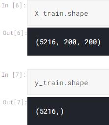
Now let us return to X_train and X_test. It is important to know that the shapes of these two arrays are (5216, 200, 200) and (624, 200, 200) respectively.
At first glance, these two shapes look okay because we can use the plt.imshow() function to display them. However, this shape convolutional layer is not acceptable because it wants to take a color channel as its input.
Therefore, since the image is essentially a grayscale image, we need to add a new 1-dimensional axis, which will be recognized by the convolutional layer as the only color channel. Although its implementation is not as complicated as my explanation:
X_train = X_train.reshape(X_train.shape[0], X_train.shape[1], X_train.shape[2], 1)
X_test = X_test.reshape(X_test.shape[0], X_test.shape[1], X_test.shape[2], 1)
After running the above code, if we check the shapes of X_train and X_test at the same time, we will see that the current shapes are (5216, 200, 200, 1) and (624, 200, 200, 1) respectively.
Data expansion
The point of increasing data (or more specifically training data) is that we will increase the amount of data used for training by creating more samples (each with a certain randomness). These randomness may include translation, rotation, scaling, shearing, and flipping.
This technique can help our neural network classifier reduce overfitting, or it can make the model better generalize the data samples. Fortunately, due to the existence of ImageDataGenerator objects that can be imported from the Keras module, the implementation is very simple.
datagen = ImageDataGenerator(
        rotation_range = 10,
        zoom_range = 0.1,
        width_shift_range = 0.1,
        height_shift_range = 0.1)
Therefore, what I did in the code above is basically to set a random range.
Next, after initializing the datagen object, what we need to do is to make it match our X_train. Then, the process is subsequently applied by the flow() method, which is very useful in this step, so that the train_gen object can now generate batches of enhanced data.
datagen.fit(X_train)train_gen = datagen.flow(X_train, y_train_one_hot, batch_size=32)
CNN (Convolutional Neural Network)
Now is the time to actually build the neural network architecture. Let's start with the input layer (input1). Therefore, this layer basically obtains all image samples in the X data. Therefore, we need to ensure that the first layer accepts the exact same shape as the image size. It is worth noting that we only need to define (width, height, channel), not (sample, width, height, channel).
Thereafter, this input layer is connected to several pairs of convolutional pool layers, and then finally connected to the fully connected layer. Please note that since the calculation speed of ReLU is faster than the S-type, all hidden layers in the model use the ReLU activation function, so the training time required is shorter. Finally, the last layer to be connected is output1, which consists of 3 neurons with softmax activation function.
The softmax is used here because we want the output to be the probability value of each category.
input1 = Input(shape=(X_train.shape[1], X_train.shape[2], 1))
cnn = Conv2D(16, (3, 3), activation='relu', strides=(1, 1),
    padding='same')(input1)
cnn = Conv2D(32, (3, 3), activation='relu', strides=(1, 1),
    padding='same')(cnn)
cnn = MaxPool2D((2, 2))(cnn)
cnn = Conv2D(16, (2, 2), activation='relu', strides=(1, 1),
    padding='same')(cnn)
cnn = Conv2D(32, (2, 2), activation='relu', strides=(1, 1),
    padding='same')(cnn)
cnn = MaxPool2D((2, 2))(cnn)
cnn = Flatten()(cnn)cnn = Dense(100, activation='relu')(cnn)
cnn = Dense(50, activation='relu')(cnn)
output1 = Dense(3, activation='softmax')(cnn)
model = Model(inputs=input1, outputs=output1)
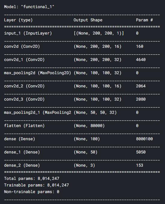
After constructing the neural network with the above code, we can display the summary of the model by applying summary() to the model object. Below are the details of our CNN model. We can see that we have a total of 8 million parameters-which is indeed a lot. Okay, that's why I run this code on Kaggle Notebook.
In short, after building the model, we need to use the classification cross-entropy loss function and the Adam optimizer to compile the neural network. Use this loss function because it is only a commonly used function in multi-class classification tasks. At the same time, I chose Adam as the optimizer because it is the best choice to minimize loss in most neural network tasks.
model.compile(loss='categorical_crossentropy',
              optimizer='adam', metrics=['acc'])
Now it's time to train the model! Here, we will use fit_generator() instead of fit() because we will get the training data from the train_gen object. If you pay attention to the data augmentation part, you will notice that train_gen is created using X_train and y_train_one_hot. Therefore, we do not need to explicitly define the Xy pair in the fit_generator() method.
history = model.fit_generator(train_gen, epochs=30,
          validation_data=(X_test, y_test_one_hot))
The special feature of train_gen is that the training process will be completed with a certain random sample. Therefore, all the training data we have in X_train will not be directly input to the neural network. Instead, these samples will be used as the basis of the generator to generate a new image through some random transformations.
In addition, the generator produces different images in each period, which is very beneficial for our neural network classifier to better generalize the samples in the test set. The following is the training process.
Epoch 1/30
163/163 [==============================] - 19s 114ms/step - loss: 5.7014 - acc: 0.6133 - val_loss: 0.7971 - val_acc: 0.7228
.
.
.
Epoch 10/30
163/163 [==============================] - 18s 111ms/step - loss: 0.5575 - acc: 0.7650 - val_loss: 0.8788 - val_acc: 0.7308
.
.
.
Epoch 20/30
163/163 [==============================] - 17s 102ms/step - loss: 0.5267 - acc: 0.7784 - val_loss: 0.6668 - val_acc: 0.7917
.
.
.
Epoch 30/30
163/163 [==============================] - 17s 104ms/step - loss: 0.4915 - acc: 0.7922 - val_loss: 0.7079 - val_acc: 0.8045
The entire training itself took about 10 minutes on my Kaggle Notebook. So be patient! After training, we can plot the increase in accuracy score and the decrease in loss, as shown below:
plt.figure(figsize=(8,6))
plt.title('Accuracy scores')
plt.plot(history.history['acc'])
plt.plot(history.history['val_acc'])
plt.legend(['acc', 'val_acc'])
plt.show()plt.figure(figsize=(8,6))
plt.title('Loss value')
plt.plot(history.history['loss'])
plt.plot(history.history['val_loss'])
plt.legend(['loss', 'val_loss'])
plt.show()


According to the above two graphs, we can say that even if the test accuracy and loss value fluctuate during these 30 periods, the performance of the model is still improving.
Another important thing to note here is that since we applied data augmentation methods early in the project, the model will not suffer from overfitting. We can see here that in the final iteration, the accuracy of the training and test data were 79% and 80%, respectively.
Fun fact: Before implementing the data augmentation method, I got 100% accuracy on the training data and 64% accuracy on the test data, which is obviously overfitting. Therefore, we can clearly see here that increasing the training data is very effective in improving the test accuracy score, while also reducing overfitting.
Model evaluation
Now, let us have a deeper understanding of the accuracy of the test data obtained using the confusion matrix. First, we need to predict all X_tests and convert the results from the one-hot format back to their actual classification labels.
predictions = model.predict(X_test)
predictions = one_hot_encoder.inverse_transform(predictions)
Next, we can use the confusion_matrix() function like this:
cm = confusion_matrix(y_test, predictions)
It is important to note that the parameters used in the function are (actual value, predicted value). The return value of the confusion matrix function is a two-dimensional array used to store the predicted distribution. To make the matrix easier to interpret, we can use the heatmap() function in the Seaborn module to display it. By the way, the value of the class name list here is obtained according to the order returned by one_hotencoder.categories.
classnames = ['bacteria', 'normal', 'virus']plt.figure(figsize=(8,8))
plt.title('Confusion matrix')
sns.heatmap(cm, cbar=False, xticklabels=classnames, yticklabels=classnames, fmt='d', annot=True, cmap=plt.cm.Blues)
plt.xlabel('Predicted')
plt.ylabel ('Actual')
plt.show()
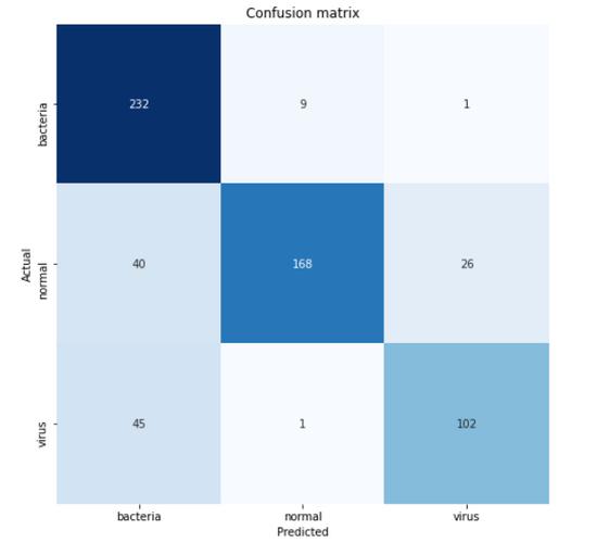
According to the confusion matrix above, we can see that 45 virus X-ray images are predicted to be bacteria. This may be because it is difficult to distinguish between the two types of pneumonia. However, at least because we correctly classified 232 of the 242 samples, our model can at least predict pneumonia caused by bacteria well.
This is the whole project! Thanks for reading! Below is all the code needed to run the whole project.
import them
import cv2import pickle    # Used to save variablesimport numpy as npimport matplotlib.pyplot as pltimport seaborn as snsfrom tqdm import tqdm    # Used to display progress bar
from sklearn.preprocessing import OneHotEncoder
from sklearn.metrics import confusion_matrix
from keras.models import Model, load_model
from keras.layers import Dense, Input, Conv2D, MaxPool2D, Flatten
from keras.preprocessing.image import ImageDataGenerator    # Used to generate images
np.random.seed(22)
# Do not forget to include the last slashdef load_normal(norm_path):    norm_files = np.array(os.listdir(norm_path))    norm_labels = np.array(['normal']*len(norm_files))
    norm_images = []    for image in tqdm(norm_files):
        # Read image        image = cv2.imread(norm_path + image)        # Resize image to 200x200 px
        image = cv2.resize(image, dsize=(200,200))
        # Convert to grayscale        image = cv2.cvtColor(image, cv2.COLOR_BGR2GRAY)        norm_images.append(image)
    norm_images = np.array(norm_images)    return norm_images, norm_labels
def load_pneumonia(pneu_path):    pneu_files = np.array(os.listdir(pneu_path))    pneu_labels = np.array([pneu_file.split('_')[1] for pneu_file in pneu_files])
    pneu_images = []    for image in tqdm(pneu_files):
        # Read image        image = cv2.imread(pneu_path + image)        # Resize image to 200x200 px
        image = cv2.resize(image, dsize=(200,200))
        # Convert to grayscale        image = cv2.cvtColor(image, cv2.COLOR_BGR2GRAY)        pneu_images.append(image)
    pneu_images = np.array(pneu_images)    return pneu_images, pneu_labels
print('Loading images')
# All images are stored in _images, all labels are in _labelsnorm_images, norm_labels = load_normal('/kaggle/input/chest-xray-pneumonia/chest_xray/train/NORMAL/')
pneu_images, pneu_labels = load_pneumonia('/kaggle/input/chest-xray-pneumonia/chest_xray/train/PNEUMONIA/')
# Put all train images to X_train X_train = np.append(norm_images, pneu_images, axis=0)
# Put all train labels to y_trainy_train = np.append(norm_labels, pneu_labels)
print(X_train.shape)
print(y_train.shape)
# Finding out the number of samples of each classprint(np.unique(y_train, return_counts=True))print('Display several images')
fig, axes = plt.subplots(ncols=7, nrows=2, figsize=(16, 4))
indices = np.random.choice(len(X_train), 14)
counter = 0
for i in range(2):
    for j in range(7):
        axes[i,j].set_title(y_train[indices[counter]])        axes[i,j].imshow(X_train[indices[counter]], cmap='gray')
        axes[i,j].get_xaxis().set_visible(False)        axes[i,j].get_yaxis().set_visible(False)        counter += 1
plt.show()print('Loading test images')
# Do the exact same thing as what we have done on train datanorm_images_test, norm_labels_test = load_normal('/kaggle/input/chest-xray-pneumonia/chest_xray/test/NORMAL/')
pneu_images_test, pneu_labels_test = load_pneumonia('/kaggle/input/chest-xray-pneumonia/chest_xray/test/PNEUMONIA/')
X_test = np.append(norm_images_test, pneu_images_test, axis=0)
y_test = np.append(norm_labels_test, pneu_labels_test)
# Save the loaded images to pickle file for future use
with open('pneumonia_data.pickle', 'wb') as f:
    pickle.dump((X_train, X_test, y_train, y_test), f)# Here's how to load it
with open('pneumonia_data.pickle', 'rb') as f:
    (X_train, X_test, y_train, y_test) = pickle.load(f)
print('Label preprocessing')
# Create new axis on all y data
y_train = y_train [:, np.newaxis]
y_test = y_test [:, e.g.newaxis]
# Initialize OneHotEncoder object
one_hot_encoder = OneHotEncoder(sparse=False)
# Convert all labels to one-hot
y_train_one_hot = one_hot_encoder.fit_transform(y_train)
y_test_one_hot = one_hot_encoder.transform(y_test)
print('Reshaping X data')
# Reshape the data into (no of samples, height, width, 1), where 1 represents a single color channel
X_train = X_train.reshape(X_train.shape[0], X_train.shape[1], X_train.shape[2], 1)
X_test = X_test.reshape(X_test.shape[0], X_test.shape[1], X_test.shape[2], 1)
print('Data augmentation')
# Generate new images with some randomness
datagen = ImageDataGenerator(
        rotation_range = 10,
        zoom_range = 0.1,
        width_shift_range = 0.1,
        height_shift_range = 0.1)
datagen.fit(X_train)
train_gen = datagen.flow(X_train, y_train_one_hot, batch_size = 32)
print('CNN')
# Define the input shape of the neural network
input_shape = (X_train.shape[1], X_train.shape[2], 1)
print(input_shape)
input1 = Input(shape=input_shape)
cnn = Conv2D(16, (3, 3), activation='relu', strides=(1, 1),
    padding='same')(input1)
cnn = Conv2D(32, (3, 3), activation='relu', strides=(1, 1),
    padding='same')(cnn)
cnn = MaxPool2D((2, 2))(cnn)
cnn = Conv2D(16, (2, 2), activation='relu', strides=(1, 1),
    padding='same')(cnn)
cnn = Conv2D(32, (2, 2), activation='relu', strides=(1, 1),
    padding='same')(cnn)
cnn = MaxPool2D((2, 2))(cnn)
cnn = Flatten()(cnn)
cnn = Dense(100, activation='relu')(cnn)
cnn = Dense(50, activation='relu')(cnn)
output1 = Dense(3, activation='softmax')(cnn)
model = Model(inputs=input1, outputs=output1)
model.compile(loss='categorical_crossentropy',
              optimizer='adam', metrics=['acc'])
# Using fit_generator() instead of fit() because we are going to use data
# taken from the generator. Note that the randomness is changing
# on each epoch
history = model.fit_generator(train_gen, epochs=30,
          validation_data=(X_test, y_test_one_hot))
# Saving model
model.save('pneumonia_cnn.h5')
print('Displaying accuracy')
plt.figure(figsize=(8,6))
plt.title('Accuracy scores')
plt.plot(history.history['acc'])
plt.plot(history.history['val_acc'])
plt.legend(['acc', 'val_acc'])
plt.show()
print('Displaying loss')
plt.figure(figsize=(8,6))
plt.title('Loss value')
plt.plot(history.history['loss'])
plt.plot(history.history['val_loss'])
plt.legend(['loss', 'val_loss'])
plt.show()
# Predicting test data
predictions = model.predict(X_test)
print(predictions)
predictions = one_hot_encoder.inverse_transform(predictions)
print('Model evaluation')
print(one_hot_encoder.categories_)
classnames = ['bacteria', 'normal', 'virus']
# Display confusion matrix
cm = confusion_matrix(y_test, predictions)
plt.figure(figsize=(8,8))
plt.title('Confusion matrix')
sns.heatmap(cm, cbar=False, xticklabels=classnames, yticklabels=classnames, fmt='d', annot=True, cmap=plt.cm.Blues)
plt.xlabel('Predicted')
plt.ylabel ('Actual')
plt.show()
Click here to get the complete project code