Machine Learning Experiment4: Logistic Regression and Newton's Method Detailed parsing the source code

1. Recalling the basic principles of Logistic Regression

1. About sigmoid function

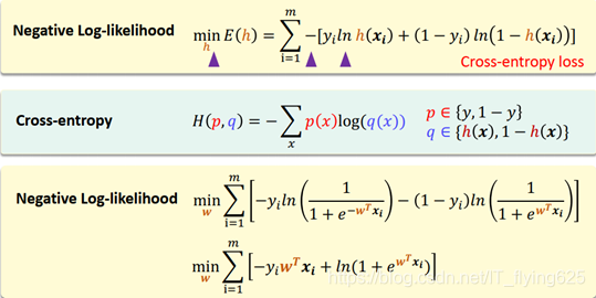
1. Maximum likelihood and loss of function

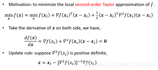
1. Newton's method

1. Experimental procedures and processes

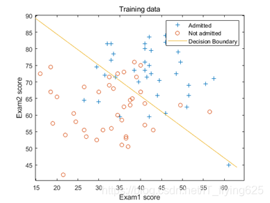
1. First, read the data and draw a scatter plot of the original data

 

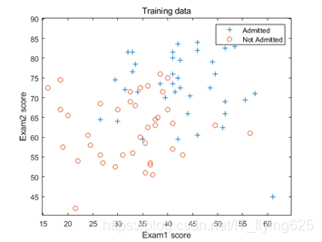
The image, we can see, the lower left mostly negative samples, and the upper right mostly positive samples, should be divided into a substantially linear negative slope.

1. The definition of predictive equations:

As used herein the sigmoid function, defined as anonymous functions (about to be eliminated because an inline function in MATLAB)

1. Defined loss function and the number of iterations

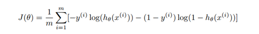
Loss function:

Parameter update rules:

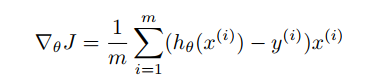
gradient:

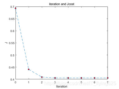
Note: where the parameter theta initialized to 0, an initial number of iterations is defined as 20, and then observe the loss function, adjusted to the appropriate number of iterations, found that when the number of iterations reaches about 6, has converged.

1. Calculation Results: iterative calculation theta

theta = zeros(n+1, 1);  %theta 3x1

iteration=8

J = zeros(iteration, 1);

for i=1:iteration

    Theta = X * Z;   % column vector 80x1 x 80x3 y 80x1  

    J(i) =(1/m)*sum(-y.*log(g(z)) - (1-y).*log(1-g(z)));

    . H = (. 1 / m) * X '* (diag (G (Z)) * diag (G (the -Z)) * X); % 3x3  is converted to a diagonal matrix

    delta=(1/m).*x' * (g(z)-y);

    theta=theta-H\delta

    %theta=theta-inv(H)*delta

end

Calculated theta value:

theta = 3×1

  -16.3787

    0.1483

    0.1589

Draw the image below:

Changes in the value of the loss function with respect to the number of iterations

prediction:

1 prediction score of 20, the results of two-dimensional probability of not being admitted 80:

prob = 1 - g([1, 20, 80]*theta)

Calculated:

prob = 0.6680

That is, the probability of not being admitted to 0.6680.

 

MATLAB source code

clc,clear
x=load('ex4x.dat')
y=load('ex4y.dat')
[m, n] = size(x);
x = [ones(m, 1), x];%增加一列
% find returns the indices of the
% rows meeting the specified condition
pos = find(y == 1); neg = find(y == 0);
% Assume the features are in the 2nd and 3rd
% columns of x
plot(x(pos, 2), x(pos,3), '+'); hold on
plot(x(neg, 2), x(neg, 3), 'o')
xlim([15.0 65.0])
ylim([40.0 90.0])
xlim([14.8 64.8])
ylim([40.2 90.2])
legend({'Admitted','Not Admitted'})
xlabel('Exam1 score')
ylabel('Exam2 score')
title('Training data')
g=@(z)1.0./(1.0+exp(-z))
% Usage: To find the value of the sigmoid 
% evaluated at 2, call g(2)
theta = zeros(n+1, 1);  %theta 3x1
iteration=8
J = zeros(iteration, 1);
for i=1:iteration
    z = x*theta;   %列向量 80x1     x 80x3   y 80x1   
    J(i) =(1/m)*sum(-y.*log(g(z)) - (1-y).*log(1-g(z)));
    H = (1/m).*x'*(diag(g(z))*diag(g(-z))*x);%3x3  转换为对角矩阵
    delta=(1/m).*x' * (g(z)-y);
    theta=theta-H\delta
    %theta=theta-inv(H)*delta
end
% Plot Newton's method result
% Only need 2 points to define a line, so choose two endpoints
plot_x = [min(x(:,2))-2,  max(x(:,2))+2];
% Calculate the decision boundary line
plot_y = (-1./theta(3)).*(theta(2).*plot_x +theta(1));
plot(plot_x, plot_y)
legend('Admitted', 'Not admitted', 'Decision Boundary')
hold off
figure
plot(0:iteration-1, J, 'o--', 'MarkerFaceColor', 'r', 'MarkerSize', 5)
xlabel('Iteration'); ylabel('J')
xlim([0.00 7.00])
ylim([0.400 0.700])
title('iteration and Jcost')
prob = 1 - g([1, 20, 80]*theta)