import pandas as pd
df = pd.read_csv('http://archive.ics.uci.edu/ml/machine-learning-databases/breast-cancer-wisconsin/wdbc.data', header=None)

from sklearn.preprocessing import LabelEncoder
X = df.loc[:, 2:].values
y = df.loc[:, 1].values
le = LabelEncoder()
y = le.fit_transform(y)

print (le.transform(['M', 'B']))

from sklearn.cross_validation import train_test_split
X_train, X_test, y_train, y_test = train_test_split(X, y, test_size=0.20, random_state=1) #数据集分为训练集和测试集
#流水线中集成数据转换及评估操作
from sklearn.preprocessing import StandardScaler
from sklearn.decomposition import PCA
from sklearn.linear_model import LogisticRegression
from sklearn.pipeline import Pipeline
pipe_lr = Pipeline([('scl', StandardScaler()),
                    ('pca', PCA(n_components=2)),
                    ('clf', LogisticRegression(random_state=1))])
pipe_lr.fit(X_train, y_train)
print('Test Accuracy: %.3f' % pipe_lr.score(X_test, y_test))

#输出
scikit-learn 分层K折交叉验 StratifiedKFold迭代器
import numpy as np
from sklearn.cross_validation import StratifiedKFold
kfold = StratifiedKFold(y=y_train,
                        n_folds=10,
                        random_state=1)
scores = []
for k, (train, test) in enumerate(kfold):
    pipe_lr.fit(X_train[train], y_train[train])
    score = pipe_lr.score(X_train[test], y_train[test])
    scores.append(score)
    print ('Fold: %s, Class dist.: %s, Acc: %.3f' % (k+1,
                                                     np.bincount(y_train[train]), score))
print ('CV accuracy: %.3f +/- %.3f' % (np.mean(scores), np.std(scores)))
scikit-learn k折交叉验证
from sklearn.cross_validation import cross_val_score
scores = cross_val_score(estimator=pipe_lr,
X=X_train,
y=y_train,
cv=10,
n_jobs=1)
print ('CV accuracy scores: %s' % scores)
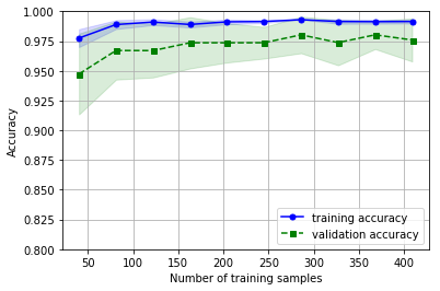
print ('CV accuracy: %.3f +/- %.3f' % (np.mean(scores), np.std(scores)))使用scikit-learn中的学习曲线函数评估模型 样本大小与训练准确率、测试准确率之间的关系
import matplotlib.pyplot as plt
from sklearn.learning_curve import learning_curve
pipe_lr = Pipeline([
('scl', StandardScaler()),
('clf', LogisticRegression(
penalty='l2', random_state=0))])
train_sizes, train_scores, test_scores = learning_curve(estimator=pipe_lr,
X=X_train,
y=y_train,
train_sizes=np.linspace(0.1, 1.0, 10),
cv=10,
n_jobs=1)
train_mean = np.mean(train_scores, axis=1)
train_std = np.std(train_scores, axis=1)
test_mean = np.mean(test_scores, axis=1)
test_std = np.std(test_scores, axis=1)
plt.plot(train_sizes, train_mean,
color='blue', marker='o',
markersize=5,
label='training accuracy')
plt.fill_between(train_sizes,
train_mean + train_std,
train_mean - train_std,
alpha=0.15, color='blue')
plt.plot(train_sizes, test_mean,
color='green', linestyle='--',
marker='s', markersize=5,
label='validation accuracy')
plt.fill_between(train_sizes,
test_mean + test_std,
test_mean - test_std,
alpha=0.15, color='green')
plt.grid()
plt.xlabel('Number of training samples')
plt.ylabel('Accuracy')
plt.legend(loc='lower right')
plt.ylim([0.8, 1.0])
plt.show()
通过验证曲线判定过拟合与欠拟合
#使用scikit-learn 绘制验证曲线 表示准确率与模型参数之间的关系

import numpy as np
from sklearn.learning_curve import validation_curve
param_range = [0.001, 0.01, 0.1, 1.0, 10.0, 100.0]
train_scores, test_scores = validation_curve(estimator=pipe_lr,
                                             X=X_train,
                                             y=y_train,
                                             param_name='clf_C',
                                             param_range=param_range,
                                             cv=10)

train_mean = np.mean(train_scores, axis=1)
train_std = np.std(train_scores, axis=1)
test_mean = np.mean(test_scores, axis=1)
test_std = np.std(test_scores, axis=1)
plt.plot(param_range, train_mean,
         color='blue', marker='o',
         markersize=5,
         label='training accuracy')
plt.fill_between(param_range, train_mean + train_std,
                 train_mean - train_std, alpha=0.15,
                 color='blue')
plt.plot(param_range, test_mean,
         color='green', linestyle='--',
         marker='s', markersize=5,
         lable='validation accuracy')
plt.fill_between(param_range,
                 test_mean + test_std,
                 test_mean - test_std,
                 alpha=0.15, color='green')

plt.grid()
plt.xscale('log')
plt.legend(loc='lower right')
plt.xlabel('Parameter C')
plt.ylabel('Accuracy')
plt.ylim([0.8, 1.0])
plt.show()