背景介绍
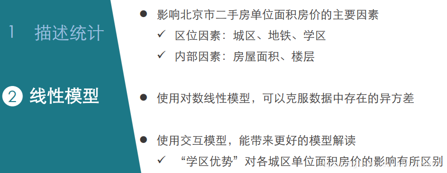
在对房价的影响因素进行模型研究之前,首先对各变量进行描述性分析,以初步判断房价的影响因素,进而建立房价预测模型
步骤如下:
(一) 因变量分析:单位面积房价分析
(二) 自变量分析:
2.1 自变量自身分布分析
2.2 自变量对因变量影响分析
(三)建立房价预测模型
3.1 线性回归模型
3.2 对因变量取对数的线性模型
3.3 考虑交互项的对数线性
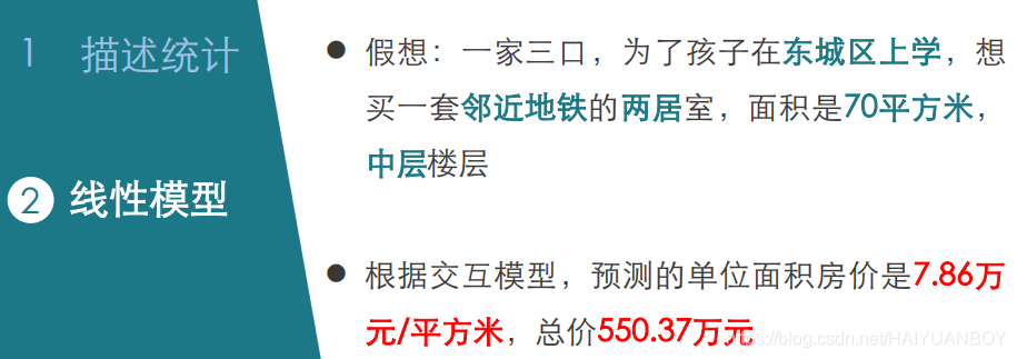
(四)预测: 假设有一家三口,父母为了能让孩子在东城区上学,想买一套邻近地铁的两居室,面积是70平方米,中层楼层,那么房价大约是多少呢?
# In[1]:
"""
dist-所在区
roomnum-室的数量
halls-厅的数量
AREA-房屋面积
floor-楼层
subway-是否临近地铁
school-是否学区房
price-平米单价
"""
# In[1]:
import pandas as pd
import numpy as np
import math
import matplotlib.pyplot as plt
import matplotlib
import seaborn as sns
import statsmodels.api as sm
from numpy import corrcoef,array
#from IPython.display import HTML, display
from statsmodels.formula.api import ols
import os
os.chdir(r"D:\pydata")
# # 1 描述
# In[17]:
datall=pd.read_csv("sndHsPr.csv") #读入清洗过后的数据
print("%d",datall.shape[0]) #样本量
#%%
#%%
dat0=datall
dat0.describe(include="all").T #查看数据基本描述
# In[18]:
dat0.price=dat0.price/10000 #价格单位转换成万元
# In[19]:
#将城区的水平由拼音改成中文,以便作图输出美观
dict1 = {
u'chaoyang' : "朝阳",
u'dongcheng' : "东城",
u'fengtai' : "丰台",
u'haidian' : "海淀",
u'shijingshan' : "石景山",
u'xicheng': "西城"
}
#%%
dat0.dist = dat0.dist.apply(lambda x : dict1[x])
dat0.head()
# 1.1 因变量
#
# price
# In[20]:
matplotlib.rcParams['axes.unicode_minus']=False#解决保存图像时负号'-'显示为方块的问题
plt.rcParams['font.sans-serif'] = ['SimHei']#指定默认字体
#因变量直方图
dat0.price.hist(bins=20)
#dat0.price.plot(kind="hist",color='lightblue')
plt.xlabel("单位面积房价(万元/平方米)")
plt.ylabel("频数")
# In[21]:
print(dat0.price.agg(['mean','median','std'])) #查看price的均值、中位数和标准差等更多信息
print(dat0.price.quantile([0.25,0.5,0.75]))
# In[22]:
#查看房价最高和最低的两条观测
pd.concat([(dat0[dat0.price==min(dat0.price)]),(dat0[dat0.price==max(dat0.price)])])
# 1.2 自变量:
#
# dist+roomnum+halls+floor+subway+school+AREA
# In[23]:
#整体来看 ,第列是连续变量,不用 value_counts,其实还可以把连续和分类变量分别放到集合里
for i in range(7):
if i != 3:
print(dat0.columns.values[i],":")
print(dat0[dat0.columns.values[i]].agg(['value_counts']).T)
print("=======================================================================")
else:
continue
print('AREA:')
print(dat0.AREA.agg(['min','mean','median','max','std']).T)
# 1.2.1 dist
# In[24]:
#频次统计
dat0.dist.value_counts().plot(kind = 'pie') #绘制柱柱形图
dat0.dist.agg(['value_counts'])
#dat0.dist.value_counts()
# In[25]:
dat0.price.groupby(dat0.dist).mean().sort_values(ascending= True).plot(kind = 'barh') #不同城区的单位房价面积均值情况
#%%
dat1=dat0[['dist','price']]
dat1.dist=dat1.dist.astype("category")
dat1.dist.cat.set_categories(["石景山","丰台","朝阳","海淀","东城","西城"],inplace=True)
#dat1.sort_values(by=['dist'],inplace=True)
sns.boxplot(x='dist',y='price',data=dat1)
#dat1.boxplot(by='dist',patch_artist=True)
plt.ylabel("单位面积房价(万元/平方米)")
plt.xlabel("城区")
plt.title("城区对房价的分组箱线图")
# In[26]:
# 1.2.2 roomnum
# In[27]:
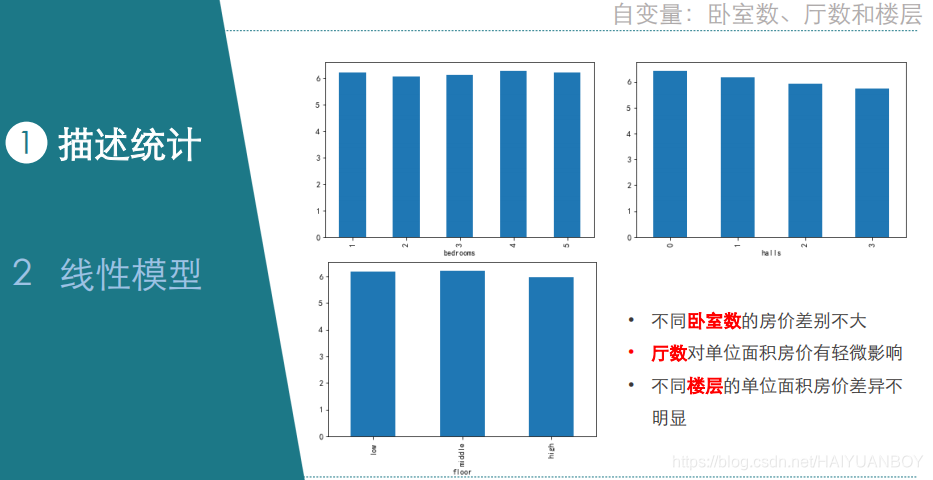
#不同卧室数的单位面积房价差异不大
dat4=dat0[['roomnum','price']]
dat4.price.groupby(dat4.roomnum).mean().plot(kind='bar')
dat4.boxplot(by='roomnum',patch_artist=True)
# 1.2.3 halls
# In[28]:
#厅数对单位面积房价有轻微影响
dat5=dat0[['halls','price']]
dat5.price.groupby(dat5.halls).mean().plot(kind='bar')
dat5.boxplot(by='halls',patch_artist=True)
# 1.2.4 floor
# In[31]:
#不同楼层的单位面积房价差异不明显
dat6=dat0[['floor','price']]
dat6.floor=dat6.floor.astype("category")
dat6.floor.cat.set_categories(["low","middle","high"],inplace=True)
dat6.sort_values(by=['floor'],inplace=True)
dat6.boxplot(by='floor',patch_artist=True)
#dat6.price.groupby(dat6.floor).mean().plot(kind='bar')
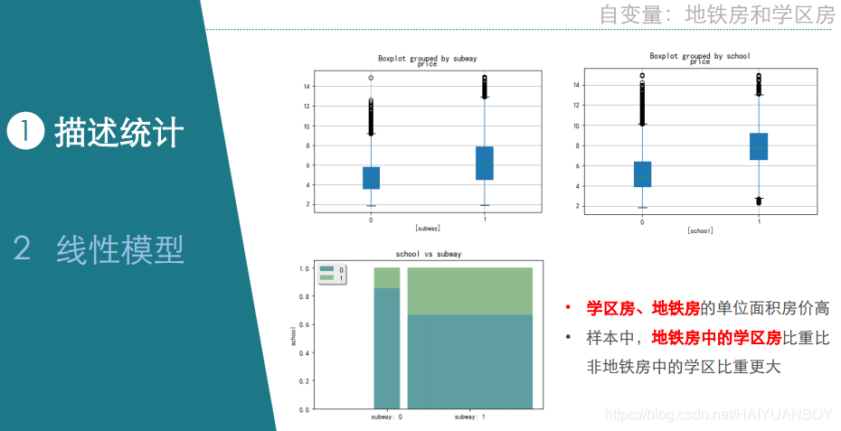
# 1.2.5 subway+school
# In[32]: 两个分类变量
print(pd.crosstab(dat0.subway,dat0.school))
sub_sch=pd.crosstab(dat0.subway,dat0.school)
sub_sch = sub_sch.div(sub_sch.sum(1),axis = 0)
sub_sch
# In[33]:
def stack2dim(raw, i, j, rotation = 0, location = 'upper left'):
'''
此函数是为了画两个维度标准化的堆积柱状图
要求是目标变量j是二分类的
raw为pandas的DataFrame数据框
i、j为两个分类变量的变量名称,要求带引号,比如"school"
rotation:水平标签旋转角度,默认水平方向,如标签过长,可设置一定角度,比如设置rotation = 40
location:分类标签的位置,如果被主体图形挡住,可更改为'upper left'
'''
import math
data_raw = pd.crosstab(raw[i], raw[j])
data = data_raw.div(data_raw.sum(1), axis=0) # 交叉表转换成比率,为得到标准化堆积柱状图
# 计算x坐标,及bar宽度
createVar = locals()
x = [0] #每个bar的中心x轴坐标
width = [] #bar的宽度
k = 0
for n in range(len(data)):
# 根据频数计算每一列bar的宽度
createVar['width' + str(n)] = data_raw.sum(axis=1)[n] / sum(data_raw.sum(axis=1))
width.append(createVar['width' + str(n)])
if n == 0:
continue
else:
k += createVar['width' + str(n - 1)] / 2 + createVar['width' + str(n)] / 2 + 0.05
x.append(k)
# 以下是通过频率交叉表矩阵生成一列对应堆积图每一块位置数据的数组,再把数组转化为矩阵
y_mat = []
n = 0
for p in range(data.shape[0]):
for q in range(data.shape[1]):
n += 1
y_mat.append(data.iloc[p, q])
if n == data.shape[0] * 2:
break
elif n % 2 == 1:
y_mat.extend([0] * (len(data) - 1))
elif n % 2 == 0:
y_mat.extend([0] * len(data))
y_mat = np.array(y_mat).reshape(len(data) * 2, len(data))
y_mat = pd.DataFrame(y_mat) # bar图中的y变量矩阵,每一行是一个y变量
# 通过x,y_mat中的每一行y,依次绘制每一块堆积图中的每一块图
createVar = locals()
for row in range(len(y_mat)):
createVar['a' + str(row)] = y_mat.iloc[row, :]
if row % 2 == 0:
if math.floor(row / 2) == 0:
label = data.columns.name + ': ' + str(data.columns[row])
plt.bar(x, createVar['a' + str(row)],
width=width[math.floor(row / 2)], label='0', color='#5F9EA0')
else:
plt.bar(x, createVar['a' + str(row)],
width=width[math.floor(row / 2)], color='#5F9EA0')
elif row % 2 == 1:
if math.floor(row / 2) == 0:
label = data.columns.name + ': ' + str(data.columns[row])
plt.bar(x, createVar['a' + str(row)], bottom=createVar['a' + str(row - 1)],
width=width[math.floor(row / 2)], label='1', color='#8FBC8F')
else:
plt.bar(x, createVar['a' + str(row)], bottom=createVar['a' + str(row - 1)],
width=width[math.floor(row / 2)], color='#8FBC8F')
plt.title(j + ' vs ' + i)
group_labels = [data.index.name + ': ' + str(name) for name in data.index]
plt.xticks(x, group_labels, rotation = rotation)
plt.ylabel(j)
plt.legend(shadow=True, loc=location)
plt.show()
# In[34]:
stack2dim(dat0, i="subway", j="school")
# In[35]:
#地铁、学区的分组箱线图
dat2=dat0[['subway','price']]
dat3=dat0[['school','price']]
dat2.boxplot(by='subway',patch_artist=True)
dat3.boxplot(by='school',patch_artist=True)
# In[35]:
# 1.2.6 AREA
#%%
datA=dat0[['AREA','price']]
plt.scatter(datA.AREA,datA.price,marker='.')
#求AREA和price的相关系数矩阵
data1=array(datA['price'])
data2=array(datA['AREA'])
datB=array([data1,data2])
corrcoef(datB)
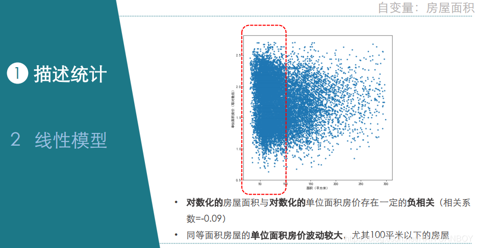
# In[58]:看到从左至右逐渐稀疏的散点图,因为是发散的,即数据右偏,第一反应是对Y取对数
#房屋面积和单位面积房价(取对数后)的散点图
datA['price_ln'] = np.log(datA['price']) #对price取对数
plt.figure(figsize=(8,8))
plt.scatter(datA.AREA,datA.price_ln,marker='.')
plt.ylabel("单位面积房价(取对数后)")
plt.xlabel("面积(平方米)")
#求AREA和price_ln的相关系数矩阵
data1=array(datA['price_ln'])
data2=array(datA['AREA'])
datB=array([data1,data2])
corrcoef(datB)
# In[58]:
#房屋面积和单位面积房价(取对数后)的散点图
datA['price_ln'] = np.log(datA['price']) #对price取对数
datA['AREA_ln'] = np.log(datA['AREA']) #对price取对数
plt.figure(figsize=(8,8))
plt.scatter(datA.AREA_ln,datA.price_ln,marker='.')
plt.ylabel("单位面积房价(取对数后)")
plt.xlabel("面积(平方米)")
#求AREA_ln和price_ln的相关系数矩阵
data1=array(datA['price_ln'])
data2=array(datA['AREA_ln'])
datB=array([data1,data2])
corrcoef(datB)
#########################################################################################
# # 2 建模
# In[38]:
#1、首先检验每个解释变量是否和被解释变量独立
#%%由于原始样本量太大,无法使用基于P值的构建模型的方案,因此按照区进行分层抽样
#dat0 = datall.sample(n=2000, random_state=1234).copy()
def get_sample(df, sampling="simple_random", k=1, stratified_col=None):
"""
对输入的 dataframe 进行抽样的函数
参数:
- df: 输入的数据框 pandas.dataframe 对象
- sampling:抽样方法 str
可选值有 ["simple_random", "stratified", "systematic"]
按顺序分别为: 简单随机抽样、分层抽样、系统抽样
- k: 抽样个数或抽样比例 int or float
(int, 则必须大于0; float, 则必须在区间(0,1)中)
如果 0 < k < 1 , 则 k 表示抽样对于总体的比例
如果 k >= 1 , 则 k 表示抽样的个数;当为分层抽样时,代表每层的样本量
- stratified_col: 需要分层的列名的列表 list
只有在分层抽样时才生效
返回值:
pandas.dataframe 对象, 抽样结果
"""
import random
import pandas as pd
from functools import reduce
import numpy as np
import math
len_df = len(df)
if k <= 0:
raise AssertionError("k不能为负数")
elif k >= 1:
assert isinstance(k, int), "选择抽样个数时, k必须为正整数"
sample_by_n=True
if sampling is "stratified":
alln=k*df.groupby(by=stratified_col)[stratified_col[0]].count().count() # 有问题的
#alln=k*df[stratified_col].value_counts().count()
if alln >= len_df:
raise AssertionError("请确认k乘以层数不能超过总样本量")
else:
sample_by_n=False
if sampling in ("simple_random", "systematic"):
k = math.ceil(len_df * k)
#print(k)
if sampling is "simple_random":
print("使用简单随机抽样")
idx = random.sample(range(len_df), k)
res_df = df.iloc[idx,:].copy()
return res_df
elif sampling is "systematic":
print("使用系统抽样")
step = len_df // k+1 #step=len_df//k-1
start = 0 #start=0
idx = range(len_df)[start::step] #idx=range(len_df+1)[start::step]
res_df = df.iloc[idx,:].copy()
#print("k=%d,step=%d,idx=%d"%(k,step,len(idx)))
return res_df
elif sampling is "stratified":
assert stratified_col is not None, "请传入包含需要分层的列名的列表"
assert all(np.in1d(stratified_col, df.columns)), "请检查输入的列名"
grouped = df.groupby(by=stratified_col)[stratified_col[0]].count()
if sample_by_n==True:
group_k = grouped.map(lambda x:k)
else:
group_k = grouped.map(lambda x: math.ceil(x * k))
res_df = df.head(0)
for df_idx in group_k.index:
df1=df
if len(stratified_col)==1:
df1=df1[df1[stratified_col[0]]==df_idx]
else:
for i in range(len(df_idx)):
df1=df1[df1[stratified_col[i]]==df_idx[i]]
idx = random.sample(range(len(df1)), group_k[df_idx])
group_df = df1.iloc[idx,:].copy()
res_df = res_df.append(group_df)
return res_df
else:
raise AssertionError("sampling is illegal")
# In[62]: 每个区抽 400 个,应该多抽几次尝试,因为有时候会抽偏
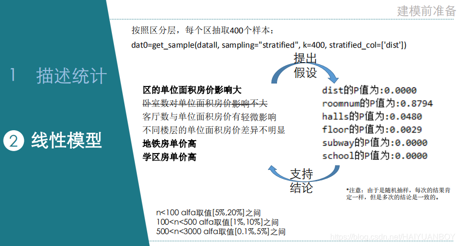
dat01=get_sample(dat0, sampling="stratified", k=400, stratified_col=['dist'])
#%%
#逐个检验变量的解释力度
"""
不同卧室数的单位面积房价差异不大
客厅数越多,单位面积房价递减
不同楼层的单位面积房价差异不明显
地铁房单价高
学区房单价高
"""
"""大致原则如下(自然科学取值偏小、社会科学取值偏大):
n<100 alfa取值[0.05,0.2]之间
100<n<500 alfa取值[0.01,0.1]之间
500<n<3000 alfa取值[0.001,0.05]之间
"""
import statsmodels.api as sm
from statsmodels.formula.api import ols
print("dist的P值为:%.4f" %sm.stats.anova_lm(ols('price ~ C(dist)',data=dat01).fit())._values[0][4])
print("roomnum的P值为:%.4f" %sm.stats.anova_lm(ols('price ~ C(roomnum)',data=dat01).fit())._values[0][4])#明显高于0.001->不显著->独立
print("halls的P值为:%.4f" %sm.stats.anova_lm(ols('price ~ C(halls)',data=dat01).fit())._values[0][4])#高于0.001->边际显著->暂时考虑
print("floor的P值为:%.4f" %sm.stats.anova_lm(ols('price ~ C(floor)',data=dat01).fit())._values[0][4])#高于0.001->边际显著->暂时考虑
print("subway的P值为:%.4f" %sm.stats.anova_lm(ols('price ~ C(subway)',data=dat01).fit())._values[0][4])
print("school的P值为:%.4f" %sm.stats.anova_lm(ols('price ~ C(school)',data=dat01).fit())._values[0][4])
#%%
###厅数不太显著,考虑做因子化处理,变成二分变量,使得建模有更好的解读
###将是否有厅bind到已有数据集
dat01['style_new']=dat01.halls
dat01.style_new[dat01.style_new>0]='有厅'
dat01.style_new[dat01.style_new==0]='无厅'
dat01.head()
# In[39]:
#
# 对于多分类变量,生成哑变量,并设置基准--完全可以在ols函数中使用C参数来处理虚拟变量,如 'price ~ C(halls)'
data=pd.get_dummies(dat01[['dist','floor']])
data.head()
# In[40]:
# 六个分类,知道5个类的值就肯定知道剩下那个类的值,所以 k 个变量,做 k-1 个哑变量
data.drop(['dist_石景山','floor_high'],axis=1,inplace=True)#这两个是参照组-在线性回归中使用C函数也可以
data.head()
# In[41]:
#生成的哑变量与其他所需变量合并成新的数据框
dat1=pd.concat([data,dat01[['school','subway','style_new','roomnum','AREA','price']]],axis=1)
dat1.head()
# 3.1 线性回归模型
# In[42]:
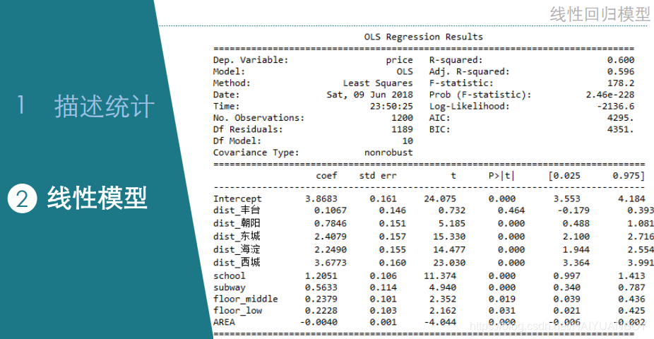
###线性回归模型
#lm1 = ols("price ~ dist_丰台+dist_朝阳+dist_东城+dist_海淀+dist_西城+school+subway+floor_middle+floor_low+style_new+roomnum+AREA", data=dat1).fit()
lm1 = ols("price ~ dist_丰台+dist_朝阳+dist_东城+dist_海淀+dist_西城+school+subway+floor_middle+floor_low+AREA", data=dat1).fit()
lm1_summary = lm1.summary()
lm1_summary #回归结果展示
#%%
"""
OLS Regression Results
==============================================================================
Dep. Variable: price R-squared: 0.593
Model: OLS Adj. R-squared: 0.591
Method: Least Squares F-statistic: 347.4
Date: Fri, 26 Apr 2019 Prob (F-statistic): 0.00
Time: 23:00:43 Log-Likelihood: -4279.5
No. Observations: 2400 AIC: 8581.
Df Residuals: 2389 BIC: 8645.
Df Model: 10
Covariance Type: nonrobust
================================================================================
coef std err t P>|t| [0.025 0.975]
--------------------------------------------------------------------------------
Intercept 3.5847 0.114 31.439 0.000 3.361 3.808
dist_丰台 0.0459 0.103 0.446 0.656 -0.156 0.248
dist_朝阳 0.8228 0.106 7.737 0.000 0.614 1.031
dist_东城 2.2936 0.110 20.890 0.000 2.078 2.509
dist_海淀 2.0530 0.108 18.949 0.000 1.841 2.265
dist_西城 3.6769 0.112 32.696 0.000 3.456 3.897
school 1.2185 0.075 16.205 0.000 1.071 1.366
subway 0.6749 0.078 8.606 0.000 0.521 0.829
floor_middle 0.1084 0.071 1.523 0.128 -0.031 0.248
floor_low 0.2802 0.073 3.848 0.000 0.137 0.423
AREA -0.0003 0.001 -0.437 0.662 -0.002 0.001
==============================================================================
Omnibus: 157.582 Durbin-Watson: 2.044
Prob(Omnibus): 0.000 Jarque-Bera (JB): 241.960
Skew: 0.531 Prob(JB): 2.88e-53
Kurtosis: 4.137 Cond. No. 671.
==============================================================================
"""
# 对于哑变量,做的时候没要哪个就跟哪个比
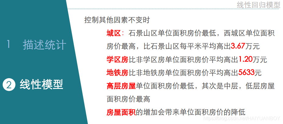
# 学区房平均比非学区房每平米贵 1.2185 万
# 中层比高层每平米贵 0.1084 万,底层比高层每平米贵 0.2802 万
# 丰台区比石景山每平米贵 0.0459 万,没什么差异,p 值为 0.656,不显著,而其他的有明显差异
#%%
lm1 = ols("price ~ C(dist)+school+subway+C(floor)+AREA", data=dat01).fit()
lm1_summary = lm1.summary()
lm1_summary #回归结果展示
# In[43]:
dat1['pred1']=lm1.predict(dat1)
# 残差
dat1['resid1']=lm1.resid
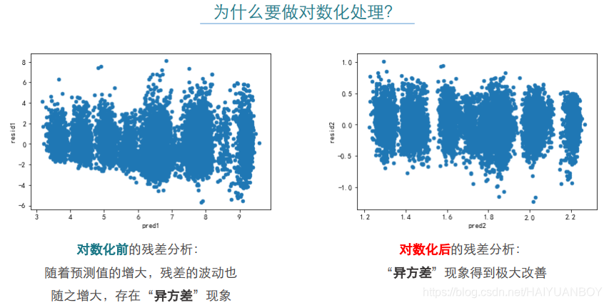
dat1.plot('pred1','resid1',kind='scatter') #模型诊断图,呈喇叭形状,存在异方差现象,对因变量取对数
# 2.2 对数线性模型
# In[44]:
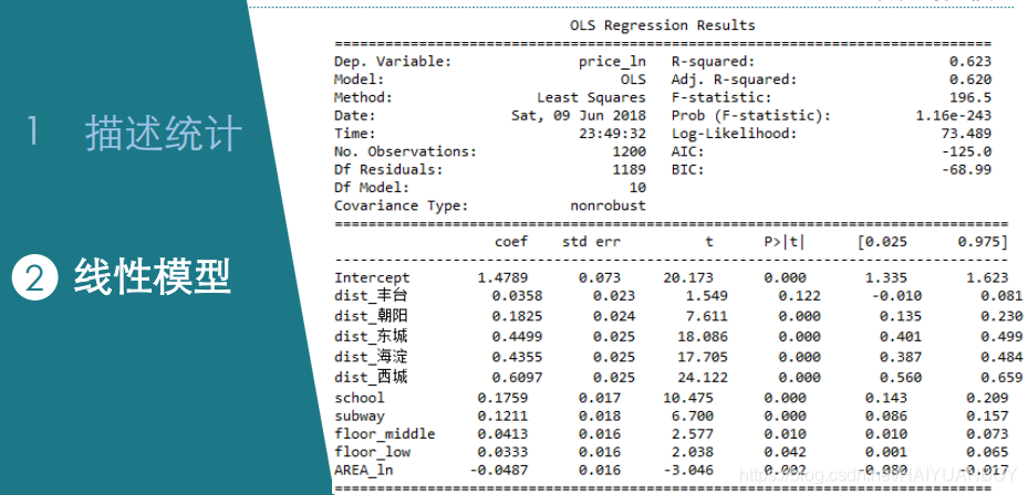
###对数线性模型
dat1['price_ln'] = np.log(dat1['price']) #对price取对数
dat1['AREA_ln'] = np.log(dat1['AREA'])#对AREA取对数
# In[45]:
lm2 = ols("price_ln ~ dist_丰台+dist_朝阳+dist_东城+dist_海淀+dist_西城+school+subway+floor_middle+floor_low+AREA", data=dat1).fit()
lm2_summary = lm2.summary()
lm2_summary #回归结果展示
# In[45]:
lm2 = ols("price_ln ~ dist_丰台+dist_朝阳+dist_东城+dist_海淀+dist_西城+school+subway+floor_middle+floor_low+AREA_ln", data=dat1).fit()
lm2_summary = lm2.summary()
lm2_summary #回归结果展示
'''
coef std err t P>|t| [0.025 0.975]
--------------------------------------------------------------------------------
Intercept 1.2979 0.054 23.960 0.000 1.192 1.404
dist_丰台 0.0316 0.017 1.885 0.060 -0.001 0.064
'''
# 取对数后解释变为丰台区比石景山每平米贵 3.16%
# In[46]:
dat1['pred2']=lm2.predict(dat1)
dat1['resid2']=lm2.resid
dat1.plot('pred2','resid2',kind='scatter') #模型诊断图,异方差现象得到消除
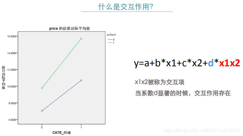
# 2.3 有交互项的对数线性模型,城区和学区之间的交互作用
# In[48]:
# In[50]:
###交互作用的解释
schools=['丰台','朝阳','东城','海淀','西城']
print('石景山非学区房\t',round(dat0[(dat0['dist']=='石景山')&(dat0['school']==0)]['price'].mean(),2),'万元/平方米\t',
'石景山学区房\t',round(dat0[(dat0['dist']=='石景山')&(dat0['school']==1)]['price'].mean(),2),'万元/平方米')
print('-------------------------------------------------------------------------')
for i in schools:
print(i+'非学区房\t',round(dat1[(dat1['dist_'+i]==1)&(dat1['school']==0)]['price'].mean(),2),'万元/平方米\t',i+'学区房\t',round(dat1[(dat1['dist_'+i]==1)&(dat1['school']==1)]['price'].mean(),2),'万元/平方米')
# In[51]:
###探索石景山学区房价格比较低的原因,是否是样本量的问题?
print('石景山非学区房\t',dat0[(dat0['dist']=='石景山')&(dat0['school']==0)].shape[0],'\t',
'石景山学区房\t',dat0[(dat0['dist']=='石景山')&(dat0['school']==1)].shape[0],'\t','石景山学区房仅占石景山所有二手房的0.92%')
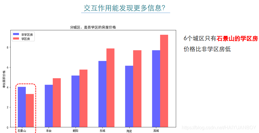
# In[52]:
###构造图形揭示不同城区是否学区房的价格问题
df=pd.DataFrame()
dist=['石景山','丰台','朝阳','东城','海淀','西城']
Noschool=[]
school=[]
for i in dist:
Noschool.append(dat0[(dat0['dist']==i)&(dat0['school']==0)]['price'].mean())
school.append(dat0[(dat0['dist']==i)&(dat0['school']==1)]['price'].mean())
df['dist']=pd.Series(dist)
df['Noschool']=pd.Series(Noschool)
df['school']=pd.Series(school)
df
# In[53]:
df1=df['Noschool'].T.values
df2=df['school'].T.values
plt.figure(figsize=(10,6))
x1=range(0,len(df))
x2=[i+0.3 for i in x1]
plt.bar(x1,df1,color='b',width=0.3,alpha=0.6,label='非学区房')
plt.bar(x2,df2,color='r',width=0.3,alpha=0.6,label='学区房')
plt.xlabel('城区')
plt.ylabel('单位面积价格')
plt.title('分城区、是否学区的房屋价格')
plt.legend(loc='upper left')
plt.xticks(range(0,6),dist)
plt.show()
# In[54]:
###分城区的学区房分组箱线图
school=['石景山','丰台','朝阳','东城','海淀','西城']
for i in school:
dat0[dat0.dist==i][['school','price']].boxplot(by='school',patch_artist=True)
plt.xlabel(i+'学区房')
# In[55]:
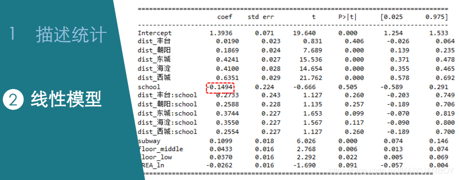
###有交互项的对数线性模型,城区和学区之间的交互作用
lm3 = ols("price_ln ~ (dist_丰台+dist_朝阳+dist_东城+dist_海淀+dist_西城)*school+subway+floor_middle+floor_low+AREA_ln", data=dat1).fit()
lm3_summary = lm3.summary()
lm3_summary #回归结果展示
'''
==================================================================================
coef std err t P>|t| [0.025 0.975]
----------------------------------------------------------------------------------
Intercept 1.3100 0.054 24.188 0.000 1.204 1.416
dist_丰台 0.0313 0.017 1.854 0.064 -0.002 0.064
dist_朝阳 0.2105 0.018 11.667 0.000 0.175 0.246
dist_东城 0.4153 0.020 20.826 0.000 0.376 0.454
dist_海淀 0.3855 0.020 19.547 0.000 0.347 0.424
dist_西城 0.6112 0.022 27.921 0.000 0.568 0.654
school -0.1715 0.136 -1.265 0.206 -0.437 0.094
dist_丰台:school 0.3105 0.147 2.106 0.035 0.021 0.600
dist_朝阳:school 0.2487 0.139 1.790 0.074 -0.024 0.521
dist_东城:school 0.3772 0.138 2.742 0.006 0.107 0.647
dist_海淀:school 0.3965 0.138 2.880 0.004 0.127 0.666
dist_西城:school 0.3533 0.138 2.567 0.010 0.083 0.623
subway 0.1238 0.013 9.715 0.000 0.099 0.149
floor_middle 0.0225 0.012 1.946 0.052 -0.000 0.045
floor_low 0.0461 0.012 3.902 0.000 0.023 0.069
AREA_ln -0.0063 0.012 -0.531 0.595 -0.030 0.017
'''
# 丰台区的学区房比非学区房每平米贵0.3105万,负的那个是石景区的
# In[55]:
###假想情形,做预测,x_new是新的自变量
x_new1=dat1.head(1)
x_new1
#%%
x_new1['dist_朝阳']=0
x_new1['dist_东城']=1
x_new1['roomnum']=2
x_new1['halls']=1
x_new1['AREA_ln']=np.log(70)
x_new1['subway']=1
x_new1['school']=1
x_new1['style_new']="有厅"
#%%
#预测值
print("单位面积房价:",round(math.exp(lm3.predict(x_new1)),2),"万元/平方米")
print("总价:",round(math.exp(lm3.predict(x_new1))*70,2),"万元")


对 price 取对数后

交互作用