参考:https://pytorch.org/tutorials/beginner/transfer_learning_tutorial.html
以下是两种主要的迁移学习场景
- 微调convnet : 与随机初始化不同,我们使用一个预训练的网络初始化网络,就像在imagenet 1000 dataset上训练的网络一样。其余的训练看起来和往常一样。
- 将ConvNet作为固定的特征提取器 : 在这里,我们将冻结所有网络的权重,除了最后的全连接层。最后一个完全连接的层被替换为一个具有随机权重的新层,并且只训练这个层。
一开始先导入需要的包:
# License: BSD
# Author: Sasank Chilamkurthy

from __future__ import print_function, division

import torch
import torch.nn as nn
import torch.optim as optim
from torch.optim import lr_scheduler
import numpy as np
import torchvision
from torchvision import datasets, models, transforms
import matplotlib.pyplot as plt
import time
import os
import copy

plt.ion()   # 交互模式
1)下载数据
将会使用torchvision和torch.utils.data包去下载数据
今天我们 要解决的问题是建立一个模型去分类蚂蚁和蜜蜂。对于蚂蚁和蜜蜂,我们分别有大约120张训练图片。对于每个类有75张验证图像。通常,如果从零开始训练,这是一个非常小的数据集。由于使用了迁移学习,我们应该能够很好地概括。
这个数据集是imagenet的一个非常小的子集。
⚠️从 here下载数据集,并将其从当前目录中抽取出来
# 为训练对数据进行扩充和规范化
# 验证只进行规范化
data_transforms = {
    'train': transforms.Compose([
        transforms.RandomResizedCrop(224),
        transforms.RandomHorizontalFlip(),
        transforms.ToTensor(),
        transforms.Normalize([0.485, 0.456, 0.406], [0.229, 0.224, 0.225])
    ]),
    'val': transforms.Compose([
        transforms.Resize(256),
        transforms.CenterCrop(224),
        transforms.ToTensor(),
        transforms.Normalize([0.485, 0.456, 0.406], [0.229, 0.224, 0.225])
    ]),
}

data_dir = './data/hymenoptera_data'
image_datasets = {x: datasets.ImageFolder(os.path.join(data_dir, x),
                                          data_transforms[x])
                  for x in ['train', 'val']}
dataloaders = {x: torch.utils.data.DataLoader(image_datasets[x], batch_size=4,
                                             shuffle=True, num_workers=4)
              for x in ['train', 'val']}
dataset_sizes = {x: len(image_datasets[x]) for x in ['train', 'val']}
class_names = image_datasets['train'].classes

#如果有CUDA则使用它,否则使用CPU
device = torch.device("cuda:0" if torch.cuda.is_available() else "cpu")
2)可视化一些图像
让我们可视化一些训练图像,以便理解数据扩充。
def imshow(inp, title=None):
    """Imshow for Tensor."""
    inp = inp.numpy().transpose((1, 2, 0))
    mean = np.array([0.485, 0.456, 0.406])
    std = np.array([0.229, 0.224, 0.225])
    inp = std * inp + mean
    inp = np.clip(inp, 0, 1)
    plt.imshow(inp)
    if title is not None:
        plt.title(title)
    plt.pause(0.001)  # 暂停一下,以便更新绘图


# 获得一批训练数据
inputs, classes = next(iter(dataloaders['train']))

# Make a grid from batch
out = torchvision.utils.make_grid(inputs)

imshow(out, title=[class_names[x] for x in classes])
运行到这里的时候就会显示如下图所示的图像:

3)训练模型
现在,让我们编写一个通用函数来训练模型。在这里,我们将举例说明:
- 调度学习比率
- 保存最佳模型
在下面,变量scheduler是一个来自torch.optim.lr_scheduler的LR调度对象,
def train_model(model, criterion, optimizer, scheduler, num_epochs=25):
    since = time.time()

    best_model_wts = copy.deepcopy(model.state_dict())
    best_acc = 0.0

    for epoch in range(num_epochs):
        print('Epoch {}/{}'.format(epoch, num_epochs - 1))
        print('-' * 10)

        # 每个周期都有一个训练和验证阶段
        for phase in ['train', 'val']:
            if phase == 'train':
                scheduler.step()
                model.train()  # 设置模型为训练模式
            else:
                model.eval()   # 设置模型为评估模式

            running_loss = 0.0
            running_corrects = 0

            #迭代数据
            for inputs, labels in dataloaders[phase]:
                inputs = inputs.to(device)
                labels = labels.to(device)

                # zero the parameter gradients
                optimizer.zero_grad()

                # forward
                # 如果只是在训练要追踪历史
                with torch.set_grad_enabled(phase == 'train'):
                    outputs = model(inputs)
                    _, preds = torch.max(outputs, 1)
                    loss = criterion(outputs, labels)

                    # backward + optimize ,仅在训练阶段
                    if phase == 'train':
                        loss.backward()
                        optimizer.step()

                # statistics
                running_loss += loss.item() * inputs.size(0)
                running_corrects += torch.sum(preds == labels.data)

            epoch_loss = running_loss / dataset_sizes[phase]
            epoch_acc = running_corrects.double() / dataset_sizes[phase]

            print('{} Loss: {:.4f} Acc: {:.4f}'.format(
                phase, epoch_loss, epoch_acc))

            # 深度拷贝模型
            if phase == 'val' and epoch_acc > best_acc:
                best_acc = epoch_acc
                best_model_wts = copy.deepcopy(model.state_dict())

        print()

    time_elapsed = time.time() - since
    print('Training complete in {:.0f}m {:.0f}s'.format(
        time_elapsed // 60, time_elapsed % 60))
    print('Best val Acc: {:4f}'.format(best_acc))

    # 下载最好的模型权重
    model.load_state_dict(best_model_wts)
    return model
4)可视化模型预测
泛型函数,显示对一些图像的预测
def visualize_model(model, num_images=6):
    was_training = model.training
    model.eval()
    images_so_far = 0
    fig = plt.figure()

    with torch.no_grad():
        for i, (inputs, labels) in enumerate(dataloaders['val']):
            inputs = inputs.to(device)
            labels = labels.to(device)

            outputs = model(inputs)
            _, preds = torch.max(outputs, 1)

            for j in range(inputs.size()[0]):
                images_so_far += 1
                ax = plt.subplot(num_images//2, 2, images_so_far)
                ax.axis('off')
                ax.set_title('predicted: {}'.format(class_names[preds[j]]))
                imshow(inputs.cpu().data[j])

                if images_so_far == num_images:
                    model.train(mode=was_training)
                    return
        model.train(mode=was_training)
5)
1》微调convent
下载预训练模型并重新设置最后的全连接层
model_ft = models.resnet18(pretrained=True)
num_ftrs = model_ft.fc.in_features
model_ft.fc = nn.Linear(num_ftrs, 2)

model_ft = model_ft.to(device)

criterion = nn.CrossEntropyLoss()

# 观察到所有参数都被优化
optimizer_ft = optim.SGD(model_ft.parameters(), lr=0.001, momentum=0.9)

# 每7个周期,LR衰减0.1倍
exp_lr_scheduler = lr_scheduler.StepLR(optimizer_ft, step_size=7, gamma=0.1)
2》训练和评估
CPU可能会使用15-25分钟。如果使用的是GPU,将花费少于一分钟
model_ft = train_model(model_ft, criterion, optimizer_ft, exp_lr_scheduler,
                       num_epochs=25)
⚠️使用的python2.7,如果使用的是python3则会报错:
(deeplearning) userdeMBP:neural transfer user$ python neural_style_tutorial.py
2019-03-13 19:30:06.194 python[4926:206321] -[NSApplication _setup:]: unrecognized selector sent to instance 0x7f8eb4895080 2019-03-13 19:30:06.199 python[4926:206321] *** Terminating app due to uncaught exception 'NSInvalidArgumentException', reason: '-[NSApplication _setup:]: unrecognized selector sent to instance 0x7f8eb4895080'
终端运行:(我是在CPU上运行的)
(deeplearning2) userdeMBP:transfer learning user$ python transfer_learning_tutorial.py
Downloading: "https://download.pytorch.org/models/resnet18-5c106cde.pth" to /Users/user/.torch/models/resnet18-5c106cde.pth
100.0%
Epoch 0/24
----------
train Loss: 0.5703 Acc: 0.7049
val Loss: 0.2565 Acc: 0.9020

Epoch 1/24
----------
train Loss: 0.6009 Acc: 0.7951
val Loss: 0.3604 Acc: 0.8627

Epoch 2/24
----------
train Loss: 0.5190 Acc: 0.7869
val Loss: 0.4421 Acc: 0.8105

Epoch 3/24
----------
train Loss: 0.5072 Acc: 0.7910
val Loss: 0.4037 Acc: 0.8431

Epoch 4/24
----------
train Loss: 0.6503 Acc: 0.7869
val Loss: 0.2961 Acc: 0.9085

Epoch 5/24
----------
train Loss: 0.3840 Acc: 0.8730
val Loss: 0.2648 Acc: 0.8954

Epoch 6/24
----------
train Loss: 0.6137 Acc: 0.7705
val Loss: 0.6852 Acc: 0.8170

Epoch 7/24
----------
train Loss: 0.4130 Acc: 0.8279
val Loss: 0.3730 Acc: 0.8954

Epoch 8/24
----------
train Loss: 0.3953 Acc: 0.8648
val Loss: 0.3300 Acc: 0.9216

Epoch 9/24
----------
train Loss: 0.2753 Acc: 0.8934
val Loss: 0.2949 Acc: 0.9020

Epoch 10/24
----------
train Loss: 0.3192 Acc: 0.8648
val Loss: 0.2984 Acc: 0.9020

Epoch 11/24
----------
train Loss: 0.2942 Acc: 0.8852
val Loss: 0.2624 Acc: 0.9150

Epoch 12/24
----------
train Loss: 0.2738 Acc: 0.8811
val Loss: 0.2855 Acc: 0.9020

Epoch 13/24
----------
train Loss: 0.2697 Acc: 0.8648
val Loss: 0.2675 Acc: 0.9020

Epoch 14/24
----------
train Loss: 0.2534 Acc: 0.9016
val Loss: 0.2780 Acc: 0.9085

Epoch 15/24
----------
train Loss: 0.2514 Acc: 0.8811
val Loss: 0.2873 Acc: 0.9020

Epoch 16/24
----------
train Loss: 0.2430 Acc: 0.9098
val Loss: 0.2901 Acc: 0.9085

Epoch 17/24
----------
train Loss: 0.2970 Acc: 0.8402
val Loss: 0.2570 Acc: 0.9150

Epoch 18/24
----------
train Loss: 0.2779 Acc: 0.8934
val Loss: 0.2792 Acc: 0.9085

Epoch 19/24
----------

train Loss: 0.2271 Acc: 0.9262
val Loss: 0.2655 Acc: 0.9150

Epoch 20/24
----------
train Loss: 0.2741 Acc: 0.8975
val Loss: 0.2726 Acc: 0.9085

Epoch 21/24
----------
train Loss: 0.3221 Acc: 0.8320
val Loss: 0.2738 Acc: 0.9150

Epoch 22/24
----------
train Loss: 0.2228 Acc: 0.9139
val Loss: 0.2712 Acc: 0.9020

Epoch 23/24
----------
train Loss: 0.2881 Acc: 0.8975
val Loss: 0.2565 Acc: 0.9150

Epoch 24/24
----------
train Loss: 0.3219 Acc: 0.8648
val Loss: 0.2669 Acc: 0.9150

Training complete in 16m 22s
Best val Acc: 0.921569
实现可视化:
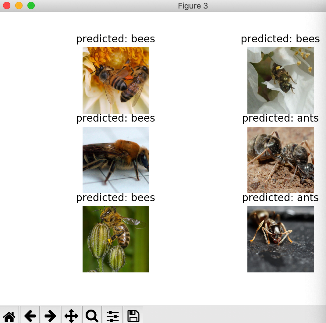
visualize_model(model_ft)
第一次返回图像为:

6)
1》将ConvNet作为固定的特征提取器
这里我们需要将除了最后一层的所有网络冻结。我们需要设置requires_grad == False去冻结参数以便梯度在backward()中不会被计算
我们可以从here读取更详细的内容
model_conv = torchvision.models.resnet18(pretrained=True)
for param in model_conv.parameters():
    param.requires_grad = False

# 最新构造函数的参数默认设置requires_grad=True
num_ftrs = model_conv.fc.in_features
model_conv.fc = nn.Linear(num_ftrs, 2)

model_conv = model_conv.to(device)

criterion = nn.CrossEntropyLoss()

# 观察到与之前相比,只有最后一层的参数被优化
optimizer_conv = optim.SGD(model_conv.fc.parameters(), lr=0.001, momentum=0.9)

# 每7个周期,LR衰减0.1倍
exp_lr_scheduler = lr_scheduler.StepLR(optimizer_conv, step_size=7, gamma=0.1)
2》训练和评估
在CPU上,与之前的场景相比,这将只花费大约其一半的时间。因为这预期了对于大部分网络梯度不需要计算。当然forward还是需要计算的
model_conv = train_model(model_conv, criterion, optimizer_conv,
                         exp_lr_scheduler, num_epochs=25)
接下来继续训练:(我是在CPU上运行的)
Epoch 0/24
----------
train Loss: 0.6719 Acc: 0.6516
val Loss: 0.2252 Acc: 0.9281

Epoch 1/24
----------
train Loss: 0.6582 Acc: 0.7254
val Loss: 0.4919 Acc: 0.7778

Epoch 2/24
----------
train Loss: 0.5313 Acc: 0.8115
val Loss: 0.2488 Acc: 0.9085

Epoch 3/24
----------
train Loss: 0.5134 Acc: 0.7623
val Loss: 0.1881 Acc: 0.9412

Epoch 4/24
----------
train Loss: 0.3834 Acc: 0.8525
val Loss: 0.2220 Acc: 0.9085

Epoch 5/24
----------
train Loss: 0.5442 Acc: 0.7910
val Loss: 0.2865 Acc: 0.8954

Epoch 6/24
----------
train Loss: 0.6136 Acc: 0.7213
val Loss: 0.2915 Acc: 0.9085

Epoch 7/24
----------
train Loss: 0.3393 Acc: 0.8730
val Loss: 0.1839 Acc: 0.9542

Epoch 8/24
----------
train Loss: 0.3616 Acc: 0.8156
val Loss: 0.1967 Acc: 0.9346

Epoch 9/24
----------
train Loss: 0.3798 Acc: 0.8402
val Loss: 0.1903 Acc: 0.9542

Epoch 10/24
----------
train Loss: 0.3918 Acc: 0.8320
val Loss: 0.1860 Acc: 0.9477

Epoch 11/24
----------
train Loss: 0.3950 Acc: 0.8115
val Loss: 0.1803 Acc: 0.9542

Epoch 12/24
----------
train Loss: 0.3094 Acc: 0.8566
val Loss: 0.1978 Acc: 0.9542

Epoch 13/24
----------
train Loss: 0.2791 Acc: 0.8811
val Loss: 0.1932 Acc: 0.9542

Epoch 14/24
----------
train Loss: 0.3797 Acc: 0.8484
val Loss: 0.2318 Acc: 0.9346

Epoch 15/24
----------
train Loss: 0.3456 Acc: 0.8689
val Loss: 0.1965 Acc: 0.9412

Epoch 16/24
----------
train Loss: 0.4585 Acc: 0.7910
val Loss: 0.2264 Acc: 0.9346

Epoch 17/24
----------
train Loss: 0.3889 Acc: 0.8566
val Loss: 0.1847 Acc: 0.9477

Epoch 18/24
----------
train Loss: 0.3636 Acc: 0.8361
val Loss: 0.2680 Acc: 0.9346

Epoch 19/24
----------
train Loss: 0.2616 Acc: 0.8730
val Loss: 0.1892 Acc: 0.9477

Epoch 20/24
----------
train Loss: 0.3114 Acc: 0.8648
val Loss: 0.2295 Acc: 0.9346

Epoch 21/24
----------
train Loss: 0.3597 Acc: 0.8443
val Loss: 0.1857 Acc: 0.9477

Epoch 22/24
----------
train Loss: 0.3794 Acc: 0.8402
val Loss: 0.1822 Acc: 0.9477

Epoch 23/24
----------
train Loss: 0.3553 Acc: 0.8279
val Loss: 0.1992 Acc: 0.9608

Epoch 24/24
----------
train Loss: 0.3514 Acc: 0.8238
val Loss: 0.2144 Acc: 0.9346

Training complete in 13m 33s
Best val Acc: 0.960784
实现可视化:
visualize_model(model_conv)

plt.ioff()
plt.show()
返回图像为: