python数据可视化: 使用matplotlib

版权声明：本文为博主原创文章，如若转载请注明出处 https://blog.csdn.net/tonydz0523/article/details/85316737

matplotlib 使用

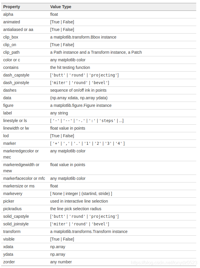
2D图属性:

import pandas as pd
import matplotlib.pyplot as plt
import numpy as np
import warnings
warnings.filterwarnings('ignore')
# 设置风格
plt.style.use('ggplot')
%matplotlib inline

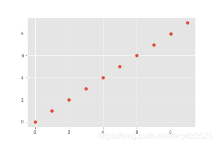
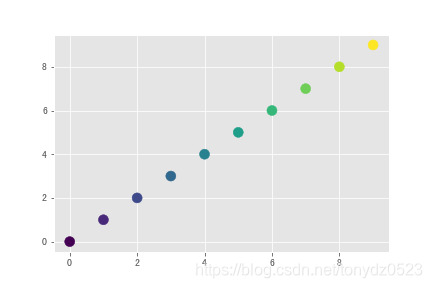
散点图

x = np.arange(10)
y = x

plt.scatter(x, y)

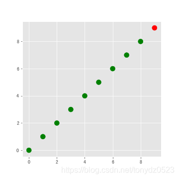
进行颜色的控制

# 颜色列表设置
colors = ['green']*(len(x)-1)
colors.append('red')

# 画幅创建 figsize调整画幅大小
plt.figure(figsize=(5,5))
# s控制大小 c控制颜色
plt.scatter(x, y, s=100, c=colors)

颜色的区分也可以根据值的不同&大小做以区分

plt.scatter(x, y, s=100, c=x)

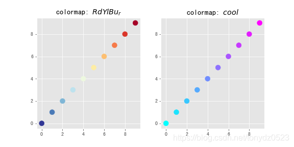
使用cmap设置颜色变换类型

# 设置画幅 nrows行数 ncols列数 cmap空值colormap选取
fig, (ax1, ax2) = plt.subplots(nrows=1, ncols=2,
                               figsize=(8, 4))
ax1.scatter(x, y, s=100, c=x, cmap='RdYlBu_r')
ax1.set_title('colormap: $RdYlBu_r$')
ax2.scatter(x, y, s=100, c=x, cmap='cool')
ax2.set_title('colormap: $cool$')

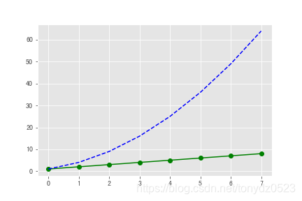
线点图

linear_data = np.array([1,2,3,4,5,6,7,8])
exponential_data = linear_data**2

# 选着线的形状颜色
plt.plot(linear_data, '-og', exponential_data, '--b')

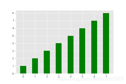
条形图

xvals = range(len(linear_data))
# 根据width控制条宽度 color空值颜色
plt.bar(xvals, linear_data, width = 0.5, color='g')

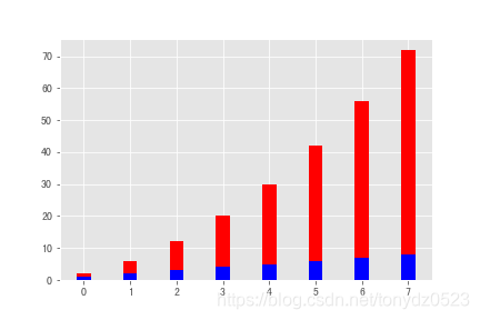
堆叠

xvals = range(len(linear_data))
plt.bar(xvals, linear_data, width = 0.3, color='b')
plt.bar(xvals, exponential_data, width = 0.3, bottom=linear_data, color='r')

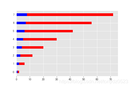
横向

xvals = range(len(linear_data))
plt.barh(xvals, linear_data, height = 0.3, color='b')
plt.barh(xvals, exponential_data, height = 0.3, left=linear_data, color='r')

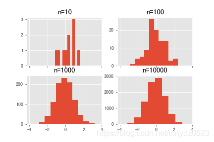
直方图

# 创造一个2x2的画布
fig, ((ax1, ax2), (ax3, ax4)) = plt.subplots(2, 2, sharex=True)
axs = [ax1,ax2,ax3,ax4]

# draw n = 10, 100, 1000, and 10000 samples from the normal distribution and plot corresponding histograms
for n in range(0,len(axs)):
    sample_size = 10**(n+1)
    sample = np.random.normal(loc=0.0, scale=1.0, size=sample_size)
    axs[n].hist(sample)
    axs[n].set_title('n={}'.format(sample_size))
    

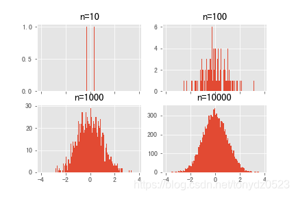
设置箱数

# 设置箱数为100
fig, ((ax1, ax2), (ax3, ax4)) = plt.subplots(2, 2, sharex=True)
axs = [ax1,ax2,ax3,ax4]
for n in range(0,len(axs)):
    sample_size = 10**(n+1)
    sample = np.random.normal(loc=0.0, scale=1.0, size=sample_size)
    axs[n].hist(sample, bins=100)
    axs[n].set_title('n={}'.format(sample_size))

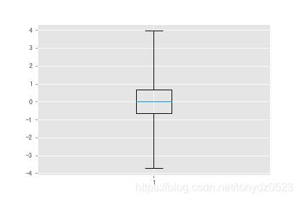
箱线图

# 数据
normal_sample = np.random.normal(loc=0.0, scale=1.0, size=10000)
random_sample = np.random.random(size=10000)
gamma_sample = np.random.gamma(2, size=10000)

df = pd.DataFrame({'normal': normal_sample, 
                   'random': random_sample, 
                   'gamma': gamma_sample})

_ = plt.boxplot(df['normal'], whis='range')

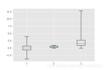
# 清理目前的画布
plt.clf()
# 三组数据同时画
_ = plt.boxplot([ df['normal'], df['random'], df['gamma'] ], whis='range')

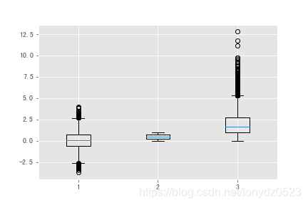
# 如果没有whis,默认为1.5倍 四分位间距IQR,可以判断离群情况
plt.figure()
_ = plt.boxplot([ df['normal'], df['random'], df['gamma'] ] )

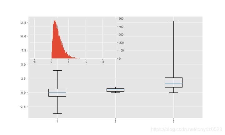
import mpl_toolkits.axes_grid1.inset_locator as mpl_il

plt.figure(figsize=(10,6))
plt.boxplot([ df['normal'], df['random'], df['gamma'] ], whis='range')
# 讲图表覆盖到另一个上
ax2 = mpl_il.inset_axes(plt.gca(), width='50%', height='40%', loc=2)
# 坐标换到右侧,避免重合
ax2.yaxis.tick_right()
ax2.hist(df['gamma'], bins=100)
ax2.margins(x=0.5)

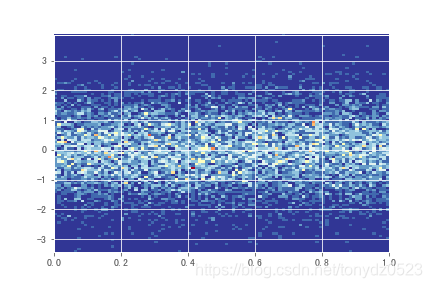
热力图

Y = np.random.normal(loc=0.0, scale=1.0, size=10000)
X = np.random.random(size=10000)
_ = plt.hist2d(X, Y, bins=25)

# 设置箱数colormap
plt.figure()
_ = plt.hist2d(X, Y, bins=100, cmap='RdYlBu_r')

饼图

labels = 'Frogs', 'Hogs', 'Dogs', 'Logs'
sizes = [15, 30, 45, 10]
# 使用expode设置hogs突出
explode = (0, 0.1, 0, 0)  # only "explode" the 2nd slice (i.e. 'Hogs')

plt.pie(sizes, explode=explode, labels=labels, autopct='%1.1f%%',
        shadow=True, startangle=90)
# 设置封宽高
plt.axis('equal')

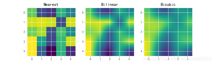
图像

A = np.random.rand(5, 5)

fig, axs = plt.subplots(1, 3, figsize=(10, 3))
for ax, interp in zip(axs, ['nearest', 'bilinear', 'bicubic']):
    ax.imshow(A, interpolation=interp)
    ax.set_title(interp.capitalize()) 
    ax.grid(True)

动图

import matplotlib.animation as animation

n = 100
x = np.random.randn(n)

# 创建要执行的函数
def update(curr):
    plt.cla()
    bins = np.arange(-4, 4, 0.5)
    plt.hist(x[:curr], bins=bins)
    plt.axis([-4,4,0,30])
    plt.annotate('n = {}'.format(curr), [3,27])

fig = plt.figure()
# update为函数, frames为帧数, interval是每一帧时间间隔为20ms
a = animation.FuncAnimation(fig, update, interval=20, frames=100)
# 保存为gif
a.save('basic_animation.gif', writer='imagemagick')

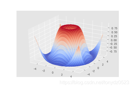
3D 图

from matplotlib import cm
from mpl_toolkits.mplot3d import Axes3D

fig = plt.figure()
ax = ax = fig.gca(projection='3d')
X = np.arange(-5, 5, 0.25)
Y = np.arange(-5, 5, 0.25)
X, Y = np.meshgrid(X, Y)
R = np.sqrt(X**2 + Y**2)
Z = np.sin(R)
surf = ax.plot_surface(X, Y, Z, rstride=1, cstride=1, cmap=cm.coolwarm)