LSTM trick之LSTMP

版权声明：本文为博主原创文章，未经博主允许不得转载。 https://blog.csdn.net/u014665013/article/details/81531620

其实在实习之前对于一些知识点的理解还是欠缺的，很多时候感觉没什么用的基础知识为什么还会在面试的时候被问到，比如，“你画一下GRU的基本结构”，你在做工程的时候回修改GRU的结构吗？居然会问这种问题哎，或许你现在也是这么想的~
但是当真正的实习的时候你会发现公司里面的数据集是需要你自己挖掘的，大公司里面的数据时很廉价的，举个例子，我之前处理的用户数据都是好几个T的，xxx亿的数据做处理，最后留下来的数据就能到5亿，这是我在实验室从来没有接触过的，几百万的数据应该就算奢侈了，但是在公司里数据可能相当的廉价。有长必有短，平时处理模型的时候你可能很少关注性能，但是公司里就不一样了，要考虑集群吃不吃得消，要考虑在多少ns ms反会结果，这样你就不得不考虑模型的大小了，另外，至少我接触到的某搜索引擎的模型都是相对比较简单的，跟我在比赛时候用的模型比起来简直是“low”到爆，为了寻求速度和效率上的提升，在基础的LSTM或者GRU中的cell上寻求一点trick也就清理之中了~
所以下次面试让你画GRU的时候，你别有什么负面情绪了，这写真的用！得！到！~
扯远了，进入今天的整体LSTMP~ show time~~~

前言

首先最简单的LSTM结构可以详见我之前的帖子（GRU和LSTM总结），但是在之后撸代码的时候我发现一个经典的LSTM结构是这样的

$$i_t=\delta(W_{ix}x_t+W_{im}m_{t-1}+W_{ic}c_{t-1}+b_i)$$

$$f_t=\delta(W_{fx}x_t+W_{fm}m_{t-1}+W_{fc}c_{t-1}+b_i)$$

$$c_t=f_t\odot c_{t-1}+i_t\odot g(W_{cx}x_t+W_{cm}m_{t-1}+b_c)$$

$$o_t=\delta(W_{ox}x_t+W_{om}m_{t-1}+W_{oc}c_{t}+b_o)$$

$$m_t=o_t\odot h(c_t)$$

$$y_t=\phi (W_{ym}m_t+b_y)$$

where the W terms denote weight matrices (e.g. Wix is the matrix of weights from the input gate to the input), $W_{ic}$, $W_{fc}$, $W_{oc}$ are diagonal weight matrices for peephole connections, the b terms denote bias vectors (bi is the input gate bias vector), σ is
the logistic sigmoid function, and i, f, o and c are respectively the input gate, forget gate, output gate and cell activation vectors, all of which are the same size as the cell output activation vector m, is the element-wise product of the vectors, g and h are the cell input and cell output activation functions, generally and in this paper tanh, and φ is the network output activation function, softmax in this paper.
—from Long Short-Term Memory Recurrent Neural Network Architectures
for Large Scale Acoustic Modeling
其实最原始的paper是long short-term memory based recurrent neural network architectures for large vocabulary speech recognition，但是你会发现在介绍参数的时候还没有上一篇讲的清楚。这里注意下$W_{ic}$, $W_{fc}$, $W_{oc}$都是对角矩阵！！！

细心的读者肯定能发现这个表达形式和我之前介绍LSTM博客在表达形式和结构上都有些区别，对于表达形式都是换汤不换药，但是这里结构上也发生了一定的变化，增加了几项：$+W_{ic}c_{t-1} 、+W_{fc}c_{t-1} 、 +W_{oc}c_{t}$
根据这个变化，我们再来回忆一下两个结构的不同：

基础版

升级版(peephole connections)

例如：即便是LSTM也有很多个变种。一个变种方式是调控门的输入。例如下面两种gate：
$g= sigmoid(W_{xg} \cdot x_t + W_{hg} \cdot h_{t-1} + {b})$:
这种gate的输入有当前的输入$x_t$和上一时刻的隐藏状态$h_{t-1}$， 表示gate是将这两个信息流作为控制依据而产生输出的。
$g= sigmoid(W_{xg} \cdot x_t + W_{hg} \cdot h_{t-1} +W_{cg} \cdot c_{t-1}+ {b})$:
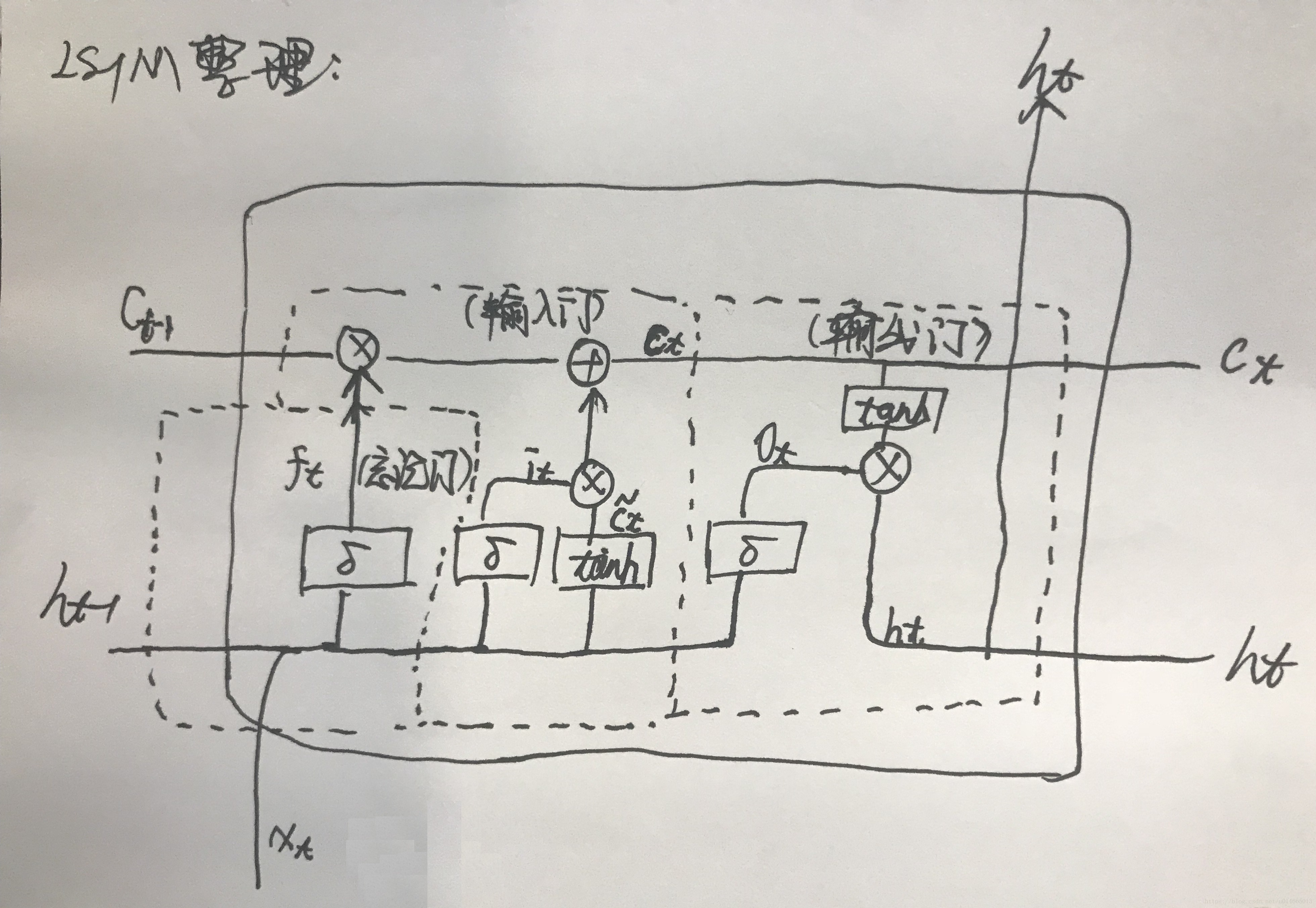
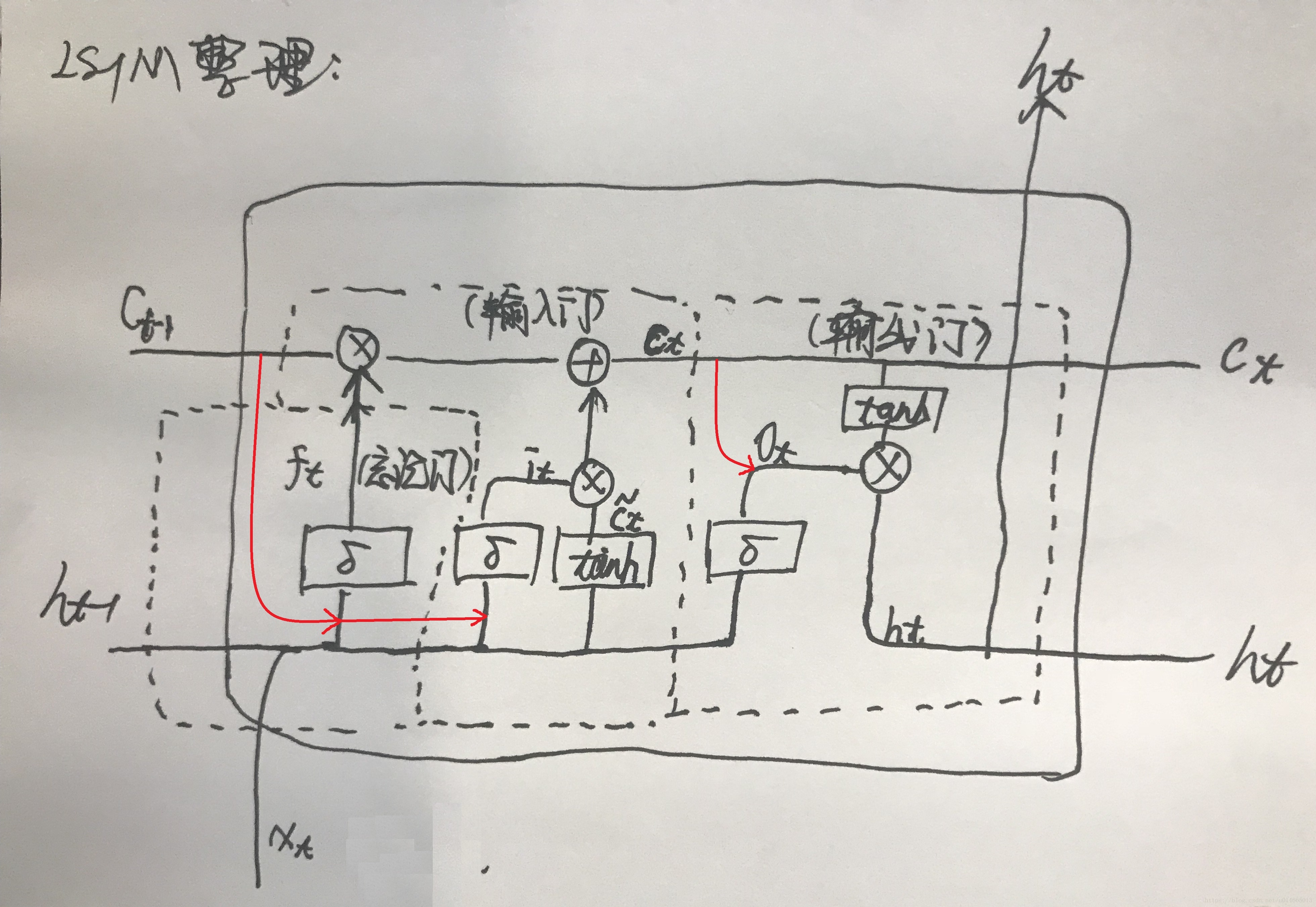
这种gate的输入有当前的输入$x_t$ 和上一时刻的隐藏状态$h_{t-1}$，以及上一时刻的cell状态$c_{t-1}$， 表示gate是将这三个信息流作为控制依据而产生输出的。这种方式的LSTM叫做peephole connections。

上面两幅图很清晰，就是在用细胞状态（就是图里面的$C_t C_{t-1}$，也就是最上面的额那条信息流）的时候有些区别。（leader说第二种的这种结构效果会比之前博客中写到的简单LSTM效果要好，我并没有试过。。。）

在下面的讲解中用到的就是第二种这个，来对比参数等一些区别。

为什么要用projection layer

首先在LSTM中的Projection layer是为了减少计算量的，它的作用和全连接layer很像，就是对输出向量做一下压缩，从而能把高纬度的信息降维，减小cell unit的维度，从而减小相关参数矩阵的参数数目！
一个很好的解释，What is the meaning of ‘projection layer’ in lstm?

传统LSTM

如上面所列出的一样，传统的LSTM的结构为：

$$i_t=\delta(W_{ix}x_t+W_{im}m_{t-1}+W_{ic}c_{t-1}+b_i)$$

$$f_t=\delta(W_{fx}x_t+W_{fm}m_{t-1}+W_{fc}c_{t-1}+b_i)$$

$$c_t=f_t\odot c_{t-1}+i_t\odot g(W_{cx}x_t+W_{cm}m_{t-1}+b_c)$$

$$o_t=\delta(W_{ox}x_t+W_{om}m_{t-1}+W_{oc}c_{t}+b_o)$$

$$m_t=o_t\odot h(c_t)$$

$$y_t=\phi (W_{ym}m_t+b_y)$$
最后的 $y_t$是输出， 公式里面的所有$m_t$表示的是图中的$h_t$，其他所有的m变成h即可，只不过写法不同而已！
那么如果不计算里面的bias（也就是 $b_i b_c b_o$），那么最终的参数数目是：
$$W=n_c*n_c*4+n_i*n_c*4+n_c*n_o+n_c*3$$
其中 $n_c$表示cell units的大小，也就是隐层的维度， $n_i$是当前输入向量的维度， $n_o$表示的是最终 $m_t$得到的最终输出y的维度
$n_c*n_c*4$表示的是 $W_{im}$、 $W_{fm}$、 $W_{cm}$、 $W_{om}$的参数个数
$n_i*n_c*4$表示的是 $W_{ix}$、 $W_{fx}$、 $W_{cx}$、 $W_{ox}$的参数个数
$n_c*n_o$表示的是 $W_{ym}$输出的时候的全连接层的参数个数
$n_c*3$表示的是 $W_{ic}$、 $W_{fc}$、 $W_{oc}$这几个 对角矩阵的参数个数

LSTM projection layer 结构（LSTMP）

而加入projection layer改进后的公式结构如下：

$$i_t=\delta(W_{ix}x_t+W_{ir}r_{t-1}+W_{ic}c_{t-1}+b_i)$$

$$f_t=\delta(W_{fx}x_t+W_{fr}r_{t-1}+W_{fc}c_{t-1}+b_i)$$

$$c_t=f_t\odot c_{t-1}+i_t\odot g(W_{cx}x_t+W_{cr}r_{t-1}+b_c)$$

$$o_t=\delta(W_{ox}x_t+W_{or}r_{t-1}+W_{oc}c_{t}+b_o)$$

$$m_t=o_t\odot h(c_t)$$

$$r_t=W_{rm}m_t$$

$$y_t=\phi (W_{yr}r_t+b_y)$$
这里的参数个数发生了变化，参数为：
$$W=n_c*n_r*4+n_i*n_c*4+n_r*n_o+n_c*n_r+n_c*3$$
其中 $n_c$表示cell units的大小，也就是隐层的维度， $n_i$是当前输入向量的维度， $n_o$表示的是最终 $m_t$得到的最终输出y的维度， $n_r$表示的是projection layer的输出维度。
$n_c*n_r*4$表示的是 $W_{im}$、 $W_{fm}$、 $W_{cm}$、 $W_{om}$的参数个数
$n_i*n_c*4$表示的是 $W_{ix}$、 $W_{fx}$、 $W_{cx}$、 $W_{ox}$的参数个数
$n_c*n_o$表示的是 $W_{ym}$输出的时候的全连接层的参数个数
$n_c*n_r$表示的是projection layer的参数矩阵
$n_c*3$表示的是 $W_{ic}$、 $W_{fc}$、 $W_{oc}$这几个 对角矩阵的参数个数

所以最终在举个例子，假设我们的cell units的大小是256，输入的维数是100，输出的维数是30，那么传统的LSTM参数个数是：

$$W=n_c*n_c*4+n_i*n_c*4+n_c*n_o+n_c*3 = 256*256*4+100*256*4+256*30+256*3 = 256*1457$$
但是加入projection layer之后，假设输出维度为128，的参数个数是：
$$W=n_c*n_r*4+n_i*n_c*4+n_r*n_o+n_c*n_r+n_c*3 = 256*128*4 + 100*256*4+128*30+256*128+256*3$$
所以减少的个数可以很容易看出来了。
相关细节未完待续！

参考网址

• lstm(三) 模型压缩lstmp
• Long Short-Term Memory Recurrent Neural Network Architectures for Large Scale Acoustic Modeling
• long short-term memory based recurrent neural network architectures for large vocabulary speech recognition
• What is the meaning of ‘projection layer’ in lstm?