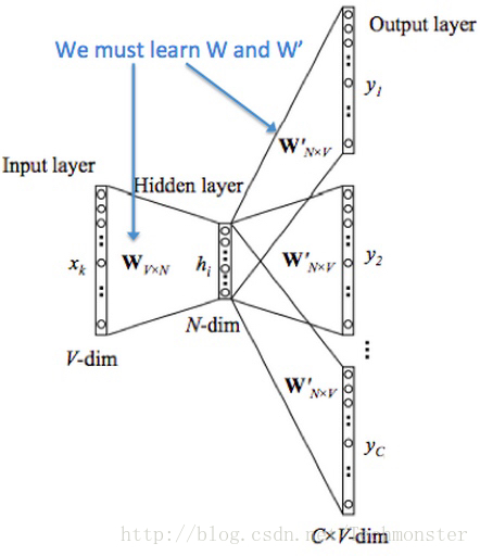
3.3 Skip-Gram Model
Another approach is to create a model such that use the center word to generate the context.
Let’s discuss the Skip-Gram model above. The setup is largely the same but we essentially swap our
x
and
y
i.e.
x
in the CBOW are now
y
and viceversa. The input one hot vector (center word) we will represent with an
x
(since there is only one). And the output vectors as
y(j)
. We define
,
the same as in CBOW.
How does it work:
1. We get our embedded word vectors for the center word:
vc=x∈ℝ|V|
2. Generate a score vector
z=vc
. As the dot product of similar vectors is higher, it will push similar words close to each other in order to achieve a high score.
4. Turn the scores into probabilities
yˆ=softmax(z)∈ℝ|V|
.
5. We desire our probabilities generated
yˆ
to match the true probabilities, the one hot vector of the actual output.
minimize J=−logP(wc−m,...,wc+m|wc)=−log∏j=0,j≠m2mP(uc−m+j|vc)=−log∏j=0,j≠m2mexp(uTcvc)∑|V|j=1exp(uTjvc)=−∑j=0,j≠m2muTc−m+jvc+2mlog∑j=1|V|exp(uTjvc)
Note that
J=−∑j=0,j≠m2mlogP(uc−m+j|vc)=−∑j=0,j≠m2mH(yˆ,yc−m+j)
Where
H(yˆ,yc−m+j)
is the cross-entropy between the probability vector
yˆ
and the one-hot vector
yc−m+j
Skip-gram treats each context word equally : the models computes the probability for each word of appearing in the context independently of its distance to the center word
shortage
Loss functions
J
for CBOW and Skip-Gram are expensive to compute because of the softmax normalization, where we sum over all
|V|
scores!
To solve this problem, a simple idea is we could instead just approximate it. We have a method called Negative Sampling
Negative Sampling
For every training step, instead of looping over the entire vocabulary, we can just sample several negative examples! We “sample” from a noise distribution (
Pn(w)
) whose probabilities match the ordering of the frequency of the vocabulary.
While negative sampling is based on Skip-Gram model or CBOW, it is in fact optimizing a different objective.
Consider a pair
(w,c)
of word and context. Did this pair came from the training data? Let’s denote by
P(D=1|w,c)
the probability that
(w,c)
came from the corpus data. Correspondingly,
P(D=0|w,c)
will be the probability that
(w,c)
did not come from the corpus data. Model
P(D=1|w,c)
with the sigmoid function:
P(D=1|w,c,θ)=σ(uTcvw)
Now, we build a new objective function that tries to maximize the probability of a word and context being in the corpus data if it indeed is, and maximize the probability of a word and context not being in the corpus data if it indeed is not. We take a simple maximum likelihood approach of these two probabilities. (Here we take
θ
to be the parameters of the model, and in our case it is
and
)
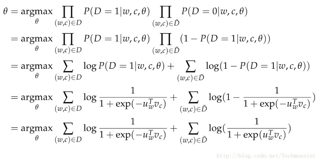
Note that maximizing the likelihood is the same as minimizing the negative log likelihood
J=−∑(w,c)∈Dlog11+exp(−uTwvc)−∑(w,c)∈D˜log11+exp(uTwvc)
Note that
D˜
is a “false” or “negative” corpus. Where we would have sentences like “stock boil fish is toy”. Unnatural sentences that should get a low probability of ever occurring. We can generate
D˜
on the fly by randomly sampling this negative from the word bank.
For skip-gram, our new objective function for observing the context word c-m+j given the center word c would be:
−logσ(uTc−m+jvc)−∑k=1Klogσ(−u˜Tkvc)
For CBOW, our new objective function for observing the center word
uc
given the context vector
vˆ=vc−m+vc−m+1+...+vc+m2m
would be
−logσ(uTcvˆ)−∑k=1Klogσ(−u˜Tkvˆ)
In the above formulation, {
u˜Tkvˆ|k=1...K
} are sampled from
Pn(w)
. There is much discussion of what makes the best approximation, what seems to work best is the Unigram Model raised to the power of 3/4. Why 3/4? Here’s an example that might help gain some intuition:
is:0.93/4=0.92constitution:0.093/4=0.16bombastic:0.013/4=0.032
“bombastic” is now 3x more likely to be sampled while “is” only went up marginally.