1、LeNet5网络结构搭建

LeNet 即 LeNet5，由 Yann LeCun 在 1998 年提出，做为最早的卷积神经网络之一，是许多神经网络架构的起点，其网络结构如图所示。

根据以上信息，就可以根据我前面文章所总结出来的方法，在 Tensorflow 框架下利用 tf.Keras 来构建 LeNet5 模型，如图所示。

图中紫色部分为卷积层，红色部分为全连接层，模型图与代码一一对应，模型搭建具体流程如下（各步骤的实现函数这里不做赘述了，请查看我前面的文章）：

输入图像大小为 32 * 32 * 3，三通道彩色图像输入；
进行卷积，卷积核大小为 5 * 5，个数为 6，步长为 1，不进行全零填充；
将卷积结果输入 sigmoid 激活函数（非线性函数）进行激活；
进行最大池化，池化核大小为 2 * 2，步长为 2；
进行卷积，卷积核大小为 5 * 5，个数为 16，步长为 1，不进行全零填充；
将卷积结果输入 sigmoid 激活函数进行激活；
进行最大池化，池化核大小为 2 * 2，步长为 2；
输入三层全连接网络进行 10 分类。

与最初的 LeNet5 网络结构相比，这里做了一点微调，输入图像尺寸为 32 * 32 * 3，以适应 cifar10 数据集。模型中采用的激活函数有 sigmoid 和 softmax，池化层均采用最大池化，以保留边缘特征。

总体上看，诞生于 1998 年的 LeNet5 与如今一些主流的 CNN 网络相比，其结构可以说是相当简单，不过它成功地利用“卷积提取特征→全连接分类”的经典思路解决了手写数字识别的问题，对神经网络研究的发展有着很重要的意义。

2、LeNet5代码实现(使用CIFAR10数据集)

import tensorflow as tf
import os
import numpy as np
from matplotlib import pyplot as plt
from tensorflow.keras.layers import Conv2D, BatchNormalization, Activation, MaxPool2D, Dropout, Flatten, Dense
from tensorflow.keras import Model

np.set_printoptions(threshold=np.inf)

cifar10 = tf.keras.datasets.cifar10
(x_train, y_train), (x_test, y_test) = cifar10.load_data()
x_train, x_test = x_train / 255.0, x_test / 255.0
#定义模型
model=tf.keras.models.Sequential([
    Conv2D(filters=6, kernel_size=(5, 5),activation='sigmoid'),
    MaxPool2D(pool_size=(2, 2), strides=2),
    Conv2D(filters=16, kernel_size=(5, 5),activation='sigmoid'),
    MaxPool2D(pool_size=(2, 2), strides=2),
    Flatten(),
    Dense(120, activation='sigmoid'),
    Dense(84, activation='sigmoid'),
    Dense(10, activation='softmax')
])
#编译模型
model.compile(optimizer='adam',
              loss=tf.keras.losses.SparseCategoricalCrossentropy(from_logits=False),
              metrics=['sparse_categorical_accuracy'])
#读取模型
checkpoint_save_path = "./checkpoint/LeNet5.ckpt"
if os.path.exists(checkpoint_save_path + '.index'):
    print('-------------load the model-----------------')
    model.load_weights(checkpoint_save_path)
#保存模型
cp_callback = tf.keras.callbacks.ModelCheckpoint(filepath=checkpoint_save_path,
                                                 save_weights_only=True,
                                                 save_best_only=True)
#训练模型
history = model.fit(x_train, y_train, batch_size=32, epochs=5, validation_data=(x_test, y_test), validation_freq=1,
                    callbacks=[cp_callback])
#查看模型摘要
model.summary()

#将模型参数存入文本
# print(model.trainable_variables)
file = open('./weights.txt', 'w')
for v in model.trainable_variables:
    file.write(str(v.name) + '\n')
    file.write(str(v.shape) + '\n')
    file.write(str(v.numpy()) + '\n')
file.close()

###############################################    show   ###############################################

# 显示训练集和验证集的acc和loss曲线
acc = history.history['sparse_categorical_accuracy']
val_acc = history.history['val_sparse_categorical_accuracy']
loss = history.history['loss']
val_loss = history.history['val_loss']

plt.subplot(1, 2, 1)
plt.plot(acc, label='Training Accuracy')
plt.plot(val_acc, label='Validation Accuracy')
plt.title('Training and Validation Accuracy')
plt.legend()

plt.subplot(1, 2, 2)
plt.plot(loss, label='Training Loss')
plt.plot(val_loss, label='Validation Loss')
plt.title('Training and Validation Loss')
plt.legend()
plt.show()

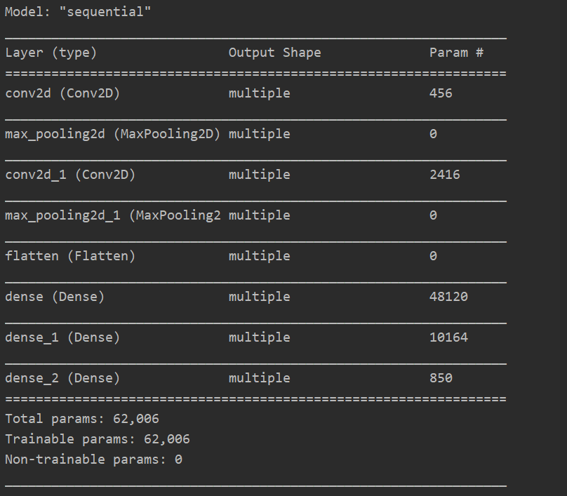
模型摘要：

经典卷积网络--LeNet

经典卷积网络--LeNet

1、LeNet5网络结构搭建

2、LeNet5代码实现(使用CIFAR10数据集)

猜你喜欢